Journal of Electromagnetic Analysis and Applications
Vol. 1 No. 4 (2009) , Article ID: 1111 , 10 pages DOI:10.4236/jemaa.2009.14030
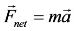
Dynamic Dipole-Dipole Magnetic Interaction and Damped Nonlinear Oscillations
![]()
University College, The Pennsylvania State University, York, USA.
Email: has2@psu.edu
Received July 10th, 2009; revised August 4th, 2009; accepted August 12th, 2009.
Keywords: Dipole-Dipole Magnetic Interaction, Damped Nonlinear Oscillations, Mathematica
ABSTRACT
Static dipole-dipole magnetic interaction is a classic topic discussed in electricity and magnetism text books. Its dynamic version, however, has not been reported in scientific literature. In this article, the author presents a comprehensive analysis of the latter. We consider two identical permanent cylindrical magnets. In a practical setting, we place one of the magnets at the bottom of a vertical glass tube and then drop the second magnet in the tube. For a pair of suitable permanent magnets characterized with their mass and magnetic moment we seek oscillations of the mobile magnet resulting from the unbalanced forces of the anti-parallel magnetic dipole orientation of the pair. To quantify the observed oscillations we form an equation describing the motion of the bouncing magnet. The strength of the magnet-magnet interaction is in proportion to the inverse fourth order separation distance of the magnets. Consequently, the corresponding equation of motion is a highly nonlinear differential equation. We deploy Mathematica and solve the equation numerically resulting in a family of kinematic information. We show our theoretical model with great success matches the measured data.
1. Introduction
It is trivial to quantify the electrostatic interaction between two point-like charges; however, in practice, it is challenging to deal with point-like charges. On the contrary, it is common practice to observe the interaction between two magnets; however, it is not that trivial to quantify their mutual interaction. For instance, the triviality of formulating the mutual interaction force between a pair of electric charge results from the fact that there are electric monopoles. We have not observed similar monopoles for the magnets thus far. The mutual magneto static interaction force between two magnets therefore is elevated beyond monopole-monopole interaction; it is considered as magnetic dipole-dipole interaction. Dipoles are geometrically extended objects. Even for planar dipoles intuitively speaking one speculates the interaction force should depend on the relative orientation of the dipoles, let alone the three dimensional configurations. As a common practice, the planar configuration is trivialized further to a one dimensional manageable situation; magnets are aligned along their mutual common axial axis [1]. Even for this configuration to the knowledge of the author there is no report utilizing its practical dynamic application. We fill in the missing gap, and propose a practical research project.
The problem is posed: Consider two permanent magnets. Position them along their mutual common axial axis and orient their magnetic moments so that are anti-parallel. Drop one of the magnets vertically on top of the second stationary magnet. Select a set of suitable characteristics for the magnets, namely the mass of the falling magnet and their magnetic moments, such that the balance between the weight of the falling magnet and the mutual magnetic force between the two magnets results in oscillations. Model the problem theoretically and confirm the accuracy of the model vs. data.
The analysis of the proposed project embodies a variety of experimental and theoretical challenges. The paper is organized to address both aspects and is composed of five sections. In Section 2, we brief the theoretical foundation evaluating the needed axial magnetic field of a permanent magnet and the magnetic force of two interacting magnets. In Section 3, guided by the theoretical insight of Section 2, we utilize two independent experimental methods and measure the needed magnetic dipole moment of the magnets. In this section we explain also the actual experiment of the bouncing magnet. In Section 4, we lay the foundation for the theoretical model and compare our model to data. In Section 5, we construct a few useful phase diagrams and in Section 6, we address the energy related issues. We close the paper with concluding remarks.
In summary, the project was stemmed from a hypothetical conceptual thought experiment. The paper is written descriptively and navigates the reader through the challenges that faced the author. To transit from a thought experiment to reality, suitable magnets had to be sought, experimental methods had to be explored, data acquisition system had to be utilized, and theoretical models had to be investigated. The proposed problem lends itself as a comprehensive physics research project. The paper provides a road map resolving the issues of interest and proves the usefulness of Mathematica [2] as a valuable research tool. From the view of the author, Mathematica to a theorist is what data acquisition utilities are to an experimentalist.
2. Axial Magnetic Field of a Permanent Magnet and Dipole-Dipole Magnetic Interaction
Magnetic field  at a distance z from the center of a counter clockwise steady current i, looping in a horizontal circle of radius R along the symmetry axis z perpendicular to the loop according to Biot-Savart law trivially evaluates [1],
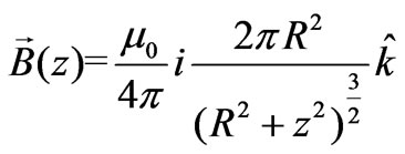 (1)
(1)
where  is the unit vector along the z-axis and
 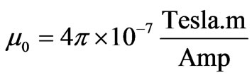 is the permeability of free space. It is customary to define
 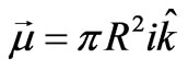 and apply Equation (1) in its entirely to a permanent magnet possessing a magnetic moment
 .
.
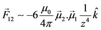
With the given quantified value of the magnetic field it is straight forward to determine the magnetic force between two permanent magnets when their moments align along their common axial axis. Viewing the interaction as being the response of the moment of one magnet to the field of the other one, the energy associated with the pair is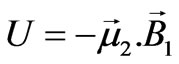 . Its spatial variation is the interaction force,
  , meaning, the force is necessitated by the inhomogeneity of the field. Utilizing Equation (1) the inhomogeneity evaluates,
 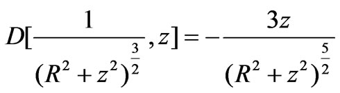 and the force becomes,
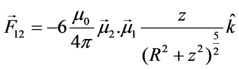 (2)
(2)
Accordingly, the anti-parallel dipole alignment results in a repulsive force and their parallel orientation provides an attractive force, respectively.
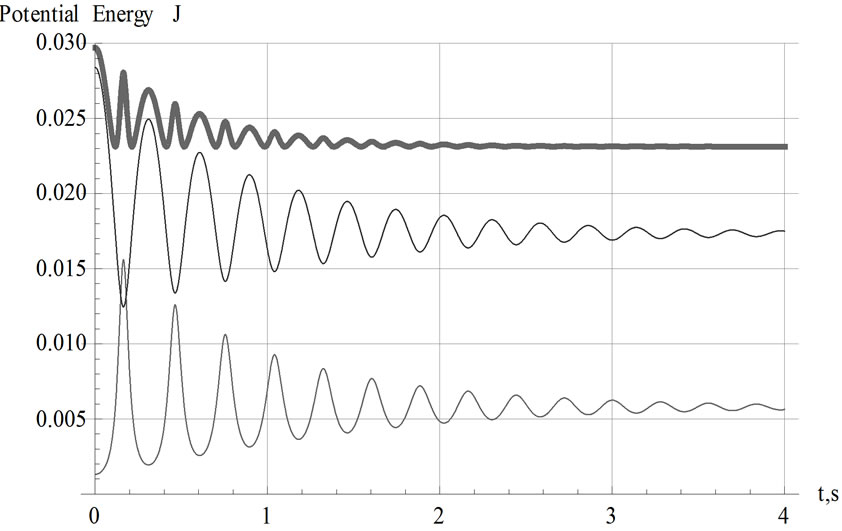
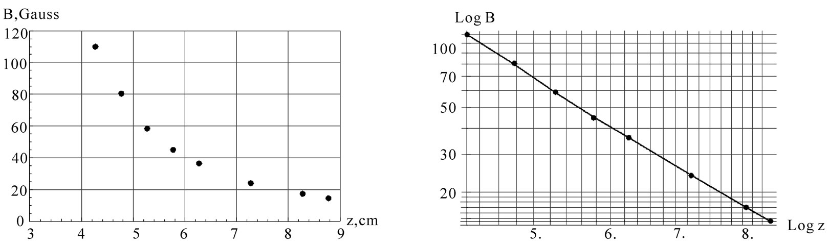
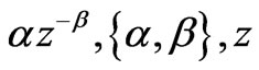
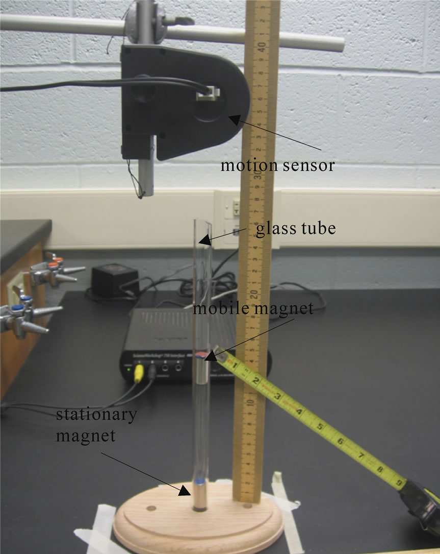
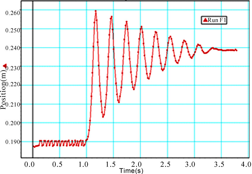
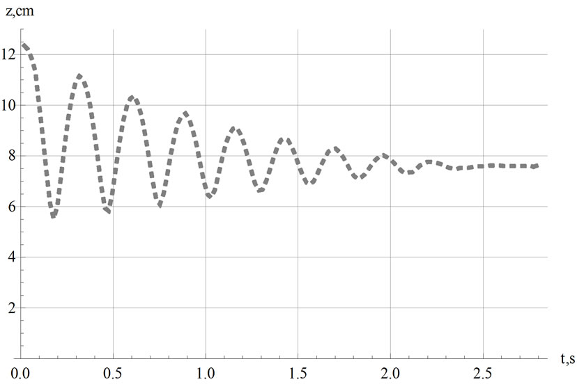
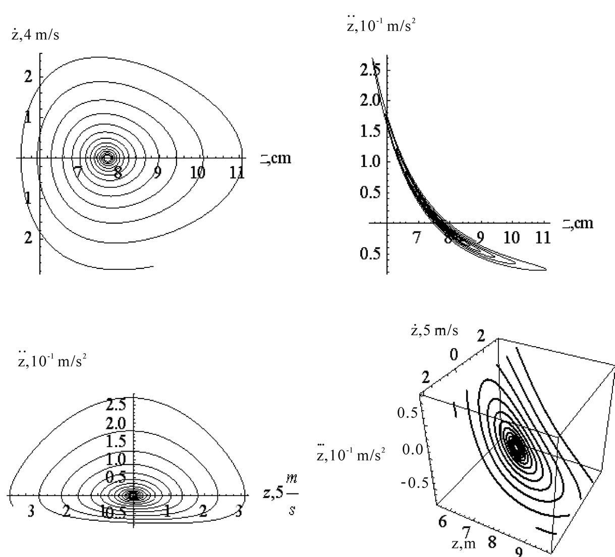
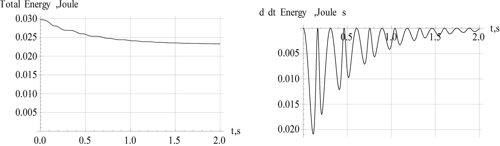
Theoretical modeling of the observed oscillations utilizes Equation (2). As we discuss in Section 4, by including other relevant forces we form an equation describing the motion of the bouncing magnet. We aim to solve the equation of motion symbolically and apply Mathematica. However, because of the highly nonlinear term of Equation (2) Mathematica provides no symbolic solution; we solve the equation numerically. Furthermore, we have observed the pair of our selected magnets always are subject to R For the chosen set of parameters describing the magnets in use, we then compare the numeric solutions of the associated equations of motion utilizing Equation (2) and Equation (4), separately; within the duration of the observed oscillations the solutions are indistinguishable. Henceforth, we utilize the simplified format of Equations (3) and (4) throughout our analysis. 3. Experimental Data 3.1 Magnetic Moment of a Permanent Magnet We acquire a variety of cylindrical magnets [3] and matching glass tubes [4].The magnets can slide freely within the tubes without touching the walls. One at a time we place the tubes containing one of the paired magnets vertically in a drilled wooden base. We run a test experiment, meaning, we drop the second magnet into the tube and see if it meaningfully bounces up and down generating data that can be documented. Among successful cases we select the pairs supporting l< To verify the practical reliability of Equation (3) we measure the field directly. Then we compare the trend of the strength of the measured field vs. distance to its theoretical counterpart, Equation (3). For our measurement we utilize Pasco™ [5] Magnetic Field Sensor/Gauss meter [6], ScienceWorkshop 750 Interface [7] and DataStudio software [8]. The first element of each Figure 1. The left plot is the display of the strength of the field vs. distance from the tip of the Gauss meter to the center of the cylinder magnet. The right graph is the log-log plot version of the left graph pair of the data set embedded in the accompanied code is the distance from the Gauss meter to the tip of the magnet in mm units; the second element is the averaged value of the measured fields in Gauss. Linear and logarithmic plots of the field vs. distance are depicted in Figure 1. The abscissa of both graphs are the distances from the tip of the Gauss meter to the center of the cylinder magnet. cylindricalMagnedata={{30,110},{35,80},{40,58.6}{45,45},{50,36},{60,24},{70,17},{75,14. 6}}/.{p_,q_}®{0.1(p+12.7),q}; plotlistdata=ListPlot[cylindricalMagnetdata,AxesLabel ®{"z,cm","B,Gauss"},PlotRange®{{3,9},{0,120}},GridLnes®Automatic,PlotStyle®{Black,PointSize[0.02]}]; lisplot1=ListLogLogPlot[cylindricalMagnetdataGridLines®Automatic,AxesLabel®{"Logz","LogB"}PlotStyle®{Black}]; listplot1=ListLogLogPlot[cylindricalMagnetdataGridLines®Automatic,AxesLabel®{"Logz","LogB"}PlotStyle®{Black}]; listplot2=ListLogLogPlot[cylindricalMagnetdataGridLines®Automatic,AxesLabel®{"Logz","LogB"}Joined®True,PlotStyle®{Black}]; s12=Show[listplot1,listplot2]; Show[GraphicsArray[{plotlistdata,s12}]] The linear plot of the raw data is depicted in the left graph of Figure 1.The right graph is the log-log display of the same data. The dimensions of the cylinder magnet are: {l,2 R}={2.54, 1.27} cm. Notably, the strongest field is measured at 3.0 cm axial distance away from the tip of the cylinder; as shown in both plots this data point falls along the general trend of the rest of the data. Utilizing the right graph of Figure 1, the slope of the slanted line measures 2.9±0.2. The slope lies within the predicted theoretical exponent of the inverse distance of Equation (3). Guided by the theoretical format of Equation (3) we fit the data applying B(z)=az-b. The plot of Log[B(z)] utilizing the fitted values of {a,b} vs. the Log[z] along with the right graph of Figure 1 is shown Figure 2. fitdata=FindFit[cylindricalMagnetdata, loglogplotfit=LogLogPlot[ Show[listplot1,loglogplotfit,s12]{a®7299.62, b®2.8922} According to our setup shown in Figure 4, for a typical run the range of the separation distance of the magnets falls within 4cm£z£8cm. Hence the small deviation of the fitted line (the tail of the dashed line) vs. data (the tail of the solid line) at distances larger than z=7.5 cm justifiably may be ignored. The values of the fitted parameters {a,b} provide two useful pieces of information. First, the slope of the fitted line is b=2.8922; as discussed, this matches the slope of the data shown in Figure 1. In other words, for our selected magnets Equation (3) justifiably is applicable. Secondly, the value of a=7299.62; hence by comparing B(z)=az-b to Equation (3) we deduce Figure 2. The solid line is the same as the right graph of Figure 1. The dashed line is the plot of the fitted function converted to MKS units, it yields m=3.65 Amp.m2. In short, the measurement of field yields the value of magnetic moment of the permanent magnet. 3.2. Magnetic Moment of a Permanent Magnet, a Static Method In this section we consider an alternate method to measure the magnetic dipole moment of a permanent magnet. Contrary to the previous method in reference to equipment, and in addition to knowing the weight of one of the magnets the only equipment needed is a straight edge. A version of this method has been discussed in [9]. The method is noble; however, without justification the authors [9] suggests to apply the approximated field of a solid disk to a set of nut-shaped magnets. On the contrary, our modified approach, as discussed in Subsection 3.1, relies on the proven consistency of theoretical approximated field given by Equation (3) vs. data. For a typical run, we place a pair of identical cylindrical magnets with their anti-parallel moments aligned along their common axial orientation in a vertical glass tube. The anti-parallel orientation of the moments causes a mutual repulsive force resulting in static equilibrium. We then measure the center-to-center separation distance of the magnets -- this yields the value of the moment. The reason is that at static equilibrium the net force on the floating magnet is zero, giving where F12 is the force of the base magnet (#1) on the suspended magnet (#2). Its value is given by Equation (4), where m is the mass of the suspended magnet. For a pair of identical magnets we solve Equation (5) for m, where z2 is the center-to-center distance of the magnets. We introduced the subscripts to identify various generalized cases -- more explanations are given in the next paragraph. We repeat of the same procedure with three identical cylindrical magnets, yielding Here, z2 and z3 are the center-to-center distances from the base to the 2nd and from the base to the 3rd magnets, respectively, and Figure 3. Four-magnet assembly setup. Magnet poles are colored red and blue Figure 4. The setup of the bouncing magnet experiment corresponding static equations for the 2nd and the 3rd magnets, respectively. Note, the first subscript of mu indicates the number of magnets for a given setup, and the second subscript corresponds to the magnet of interest. E.g. the indices of For each assembly we then measure the needed distances and apply the corresponding equations to evaluate the m’s. For each assembly we then plot the values of the moments vs. the number of the magnets. The graph reveals the distribution of moments about the overall mean value of the moments is sharp; we then objectively evaluate the mean value of each assembly and then evaluate the mean of the mean. Notice also to measure the mass of the magnet we use a balance with an accuracy of 0.1 grams. Considering the accuracy of a straight edge is 1 mm, our systematic error yields 12%; Hence, our measurement yields m=(3.58±0.43) Amp.m2. Comparing to the measurement of the previous method, although the values of the moments are comparable, it appears that we should prefer the method of the previous section. A photo of the setup for a four-magnet assembly is shown in Figure 3. (*Import["C:\\DataFiles\\MagneticDipole_Fall2008\\Cyl-indricalMagnet Nov28_2008\\IMG_2589.jpg", Image Size®{120,180}];*) 3.3. The Bouncing Magnet The experiment setup is shown in Figure 4. It consists of a pair of identical cylindrical magnets assembled in a suitable vertical glass tube. The tube is placed in a wooden drilled base. Along the extension of the tube using nonmagnetic rods and clamps we mount the Motion sensor [10] and connect it to the Interface [7]. To run the experiment (shown in Figure 4) we lift the top magnet with the metallic lip of a measuring tape and position it in the front of the motion sensor. We then activate the motion sensor and with a jolt pull the lip of the measuring tape away. The suspended magnet falls and bounces off the bottom magnet. While the top magnet oscillates up and down the motion sensor collects data; the sensor measures and stores the coordinates of the magnet along with its corresponding time. Applying DataStudio [8] we store the data set and the displayed image. One such image is shown in Figure 5. We then import the image and the data to Mathematica. (*Import["C:\\DataFiles\\MagneticDipole_Fall2008\\Cyl-indricalMagnetNov28_2008\\IMG_2594.jpg", ImageSi ze®{120,200},Alignment®{Center}];*) Import["C:\\DataFiles\\MagneticDipole_Fall2008\\Cy lindricalMagneNov28_2008\\position1_Dec4_20 08.bmp ",ImageSize®400,Alignment®{Center}] The run time of the experiment is about 2.0 s and the magnet on an average oscillates eight times with an approximate period of 0.3 s. The largest amplitude of oscillation typically is 8 cm. The closest distance of approach of the bouncing magnet from the base magnet on average is greater than 4 cm; this is within the z-3 approximation of magnetic field. 4. A Theoretical Model With the data on hand we devise our model. The basis of our model stems from dynamics, meaning, we deal with active forces. In addition to the relevant forces acting on the mobile magnet namely weight and the dipole-dipole magnetic repulsive force, we introduce a new factor, the speed dependent viscous force. The viscous coefficient for the ceramic magnet against the glass tube and the surrounding air is unknown. Therefore, our model embodies an unknown parameter. Guided with data we adjust the value of this unknown parameter; the procedure follows. Utilizing DataStudio we export the collected data to Microsoft™ Excel [11], apply ExcelLink for Mathematica [12] we import the data to Mathematica. The imported data is a list of pairs of numbers; applying Mathematica rules we manipulate the list accordingly. For instance, in accordance with the displayed data in Figure 5, we drop the extraneous irrelevant data points and convert the ordinance into MKS units. Furthermore by knowing the distance of the motion sensor from the base magnet conveniently we replace the ordinance of the raw data with the distance between the magnets. Figure 6 displays the center-to-center distance of the bouncing magnet vs. the acquired time. ExcelLink` Utilizing an active Excel file, we read the data. File:C: |DataFiles|MagneticDipole_ Fall2008|CylindricalMagnetNov28_2008|position1_Dec4_2008.xls data=ExcelRead["a7:b197"]; ListLinePlot[Drop[data,50]/.{p_,q_}®{p,100q},PlotRange®{{1,3.5},{0,30}}]; plotdata=ListLinePlot[Drop[data,50]/.{p_,q_}®{p-data[[50,1]],100(-(q+0.0254)+0.340)},PlotRange®{0,13},PlotStyle®{Dashing[{0.01},GrayLevel[0.5],Thickness [0.006]};GridLines®Automatic,AxesLabel®{“t,s”,”z,cm”}] Figure 5. The data displays the coordinates of the bouncing magnet measured from the motion sensor vs. the corresponding time Figure 6. Display of the center-to-center distance of the bouncing magnet vs. the acquired time Figure 7. Comparison of the theoretical model (the solid black line) vs. the experimental data (the dashed gray line) The graph shows the bouncing magnet gets as close as 5.5 cm of the tip of the base magnet, and it settles at 7.5 cm away from it. This justifies the applicability of Equation (3). We formulate the viscous force as Gv, where G and v are the viscous coefficient and the speed of the mobile magnet, respectively. Applying Newton’s second law, where g= values={g->9.8, eqz=z''[t]-(6(m0/(4p))meanm2)/(mz[t]4)+ gz'[t]+g/.values; solz=NDSolve[{eqz=0,z[0.0] =12.610-2,z'[0.] =0},z[t],{t,0.,4}];{positionz,speedz,accz}={z[t]/.solz[[1]],D[z[t]/.solz[[1]],t],D[z[t]/.solz[[1]],{t,2}]}; plotz=Plot[102 positionz,{t,0.,3},AxesLabel®{"t,s","z,cm"},PlotRange®{All,{0.,13}},GridLines® Automatic,PlotStyle®{Thickness[0.008],Black}]; tabz=Table[positionz,{t,0,4,0.02}];Manipulate[Show[{plotz,plotdata,Graphics[{AbsolutePointSize[6],Black,Point[{0,102 tabz[[n]]}]}]},PlotRange->{All,{0,13}}],{n,1,Length[tabz],1}] As shown in Figure 7 the model (the black solid line) fits quite well vs. the data (the dashed gray line). Figure 7 is a snapshot of the animated oscillations of the magnet -- the black disk represents the mobile magnet. The animation code given in the text allows one to run the program in an interactive mode and watch the bouncing disk along the z-axis. The model's amplitude and the period of the oscillations closely follow the data. Within 2.2 s the magnet oscillates eight times. It appears beyond 1.5 s there are somewhat insignificant differences between the Figure 8. From left to right the plots are: the oscillation amplitude, velocity, and acceleration of the bouncing magnet vs. time. For clarity purpose only we applied CGS units to the first graph and MKS units to the last two graphs Figure 9. Implicit two and three-dimensional plots of various combinations of kinematic quantities of the bouncing magnet. For the sake of displaying the graphs clearly axes are scaled by certain factors Figure 10. The left and the right graphs are the display of total energy and the rate of loss vs. time for the bouncing magnet, respectively model calculation and data. However, beyond 1.5 s the amplitudes are about 1.5 cm, and the precision of the motion sensor for this small range is questionable. The damped oscillations of the bouncing magnet shown in Figure 7 deceptively resemble the oscillations of a damped simple harmonic motion; recall that the restoring force describing the latter is a linear force. To show the impact of the nonlinear force of the former i.e z-4, we plot the velocity and acceleration of the bouncing magnet vs. time. These two graphs along with the oscillation amplitudes are depicted in Figure 8. An experienced reader would realize that the last two plots of Figure 8 distinctly are different from their counterpart of damped simple harmonic oscillations. plotspeedz=Plot[speedz,{t,10-2,4},AxesLabel®{"t,s"," plotaccz=Plot[accz,{t,10-2,4},AxesLabel®{"t,s"," Show[GraphicsArray[{plotz,plotspeedz,plotaccz}]] In practice, the magnet is released from its initial height of 12.6 cm away from the base magnet; its initial velocity and acceleration are zero and ~ -8.2m/s2, respectively. These are the ordinances of the curves depicted in the last two plots of Figure 8 at t=0. The initial acceleration is less than gravity, indicating the impact of the repulsive force exerted by the base magnet. The first graph shows the falling magnet; within 0.164 s, it reaches its closest distance of about 5.5 cm from the base magnet. At that moment, its acceleration is at its greatest, ~27 m/s2. As shown in the first graph, the process accordingly repeats itself until the loss of the oscillating amplitudes due to the viscous force, settles the magnet at its stable, at a static equilibrium height of 7.5 cm. 5. Phase Diagrams Graphs depicted in Figure 8 display various kinematic quantities of the bouncing magnet vs. time. Utilizing Mathematica we fold the time axis and display a pair of quantities such as, {positionz,speedz,accz}/.t®0.164 {0.0552837,0.00654413,26.9876} phas2Plotzv=ParametricPlot[{102 positionz,4 speedz}{t,10-1,4},AxesLabel®{"z,cm"," phas2Plotza=ParametricPlot[{102 positionz,10-1 accz}{t,10-1,3.999},AxesLabel®{"z,cm"," phas2Plotva=ParametricPlot[{5speedz, 10-1 accz},{t,10-1,3.999},AxesLabel®{" phasePlotzva=ParametricPlot3D[{102 positionz,5speedz,10-1 accz},{t,10-1,3.999},AxesLabel®{"z,m"," Show[GraphicsArray[{{phas2Plotzv,phas2Plotza},{phas2Plotva,phasePlotzva}}]] Graphs shown in Figure 9 are useful. For instance, the left upper corner graph shows the impact of the viscous force -- it is the cause of the spiral curvature. Similarly, the bottom left graph displays the relationship between acceleration and its associated velocity. 6. Energy Characteristics of the Bouncing Magnet Knowing the time dependent position of the bouncing magnet, z(t), we write its energy E=KE+U. KE is Kinetic Energy and is KE=1/2 mv2; U is potential energy and is plotTotalEnergy=Plot[Evaluate[(1/2m speedz2+2(m0/ (4p)) meanm2 1/positionz3+m g positionz)/.values]{t,0,2},PlotRange®{0,All},AxesLabel®{"t,s","Total Energy,Joule"},PlotStyle®{GrayLevel[0.2]},GridLines ®Automatic]; dEnergy=D[Evaluate[(1/2m speedz2+2(m0/(4p)) meanm2 1/positionz3+m g positionz)/.values],t]; plotdEnergy=Plot[dEnergy,{t,0,2},PlotRange®All,AxesLbel®{"t,s","d/dt(Energy),Joule/s"},PlotStyle®{Black},GridLines®Automatic]; Show[GraphicsArray[{plotTotalEnergy,plotdEnergy}]] The left graph of Figure 10 shows the bouncing magnet loses its energy over time. This is attributed to the viscous effect. Because of the smallness of the viscous force the loss over the time-span of the oscillations is small. The graph on the right panel of Figure 10 reveals Figure 11. Display of the gravitational (the dark thin gray line), magnetic (the light thin gray line) and the total (the dark thick gray line) potential energies of the bouncing magnet, vs. time Figure 12. Display of potential energy (the semi-dark thick gray line; the second curve from top), kinetic energy (light thick gray line; the bottom curve) and the total energy (the thin black line; the top curve) of the bouncing magnet vs. time, respectively. The middle thick black line is the display of the vertical position of the bouncing magnet vs. time. For convenience, the latter compared to Figuire 6 is downsized by a factor of 0.15 that the rate of the loss of energy is not uniform. To have a better understanding about the time dependent behavior of energy, we dissect the energy and look at the time variations of its composites. Figure 11 is a display of the time dependent variation of the gravitational and magnetic potential energies. plotTotalPE=Plot[(2(m0/(4p)) meanm2 1/positionz3+m gpostionz)/.values,{t,0,4},PlotStyle®{GrayLevel[0.4],Thickness[0.008]},PlotRange®{All,{0,0.03}},AxesLabel®{"t,s","TotalPE,Joule"},GridLines®Automatic]; plotGravityPE=Plot[(m g positionz)/.values,{t,0,4},PlotStyle®{GrayLevel[0.2]},PlotRange®{All,{0,0.03 }},AxesLabel®{"t,s","Gravitational PE,Joule"},GridLines®Automatic]; plotMagneticPE=Plot[(2(m0/(4p)) meanm2 1/positionz3)/.values,{t,0,4},PlotStyle®{GrayLevel[0.4]},PlotRange®{All,{0,0.03}},AxesLabel®{"t,s","Magnetic PE,Joule"},GridLines®Automatic]; Show[plotMagneticPE,plotGravityPE,plotTotalPE,AxesLabel®{"t,s","Potential Energy,Joule"}] According to Figure 11 and on a par with one's expectation, the gravitational (the dark thin gray line) and the magnetic (the light thin gray line) potential energies are completely out of synch. Meaning, initially when the magnets are farthest apart from each other, the gravity potential with respect to the base magnet is at its maximum and the magnetic potential energy is at its minimum. At the end of the fall when the magnets are at their closest distance from each other, the former reaches its minimum potential energy while the latter is at maximum. Furthermore, the time dependent variation of the gravitational potential energy by itself vs. time is less interesting; it follows the trend of the z(t). However, the time dependent variation of the magnetic potential energy has a peculiar character. Its characteristics are a finger print of the non-linearity of the force. We display collectively the various energies of the bouncing magnet in Figure 12. plotKE=Plot[(1/2 m speedz2/.values),{t,0,4},PlotStyle®{GrayLevel[0.6],Thickness[0.008]},PlotRange®{All,{0,0.006 }},AxesLabel{"t,s","KE,Joule"},GridLines®Automatic]; plotEnergy=Show[plotTotalPE,plotKE,plotTotalEnergy,AxesLabel®{"t,s","Enrgy,Jouels"},PlotRange®All]; plotz1=Plot[0.15positionz,{t,0.,3},AxesLabel®{"t,s","z,cm"},PlotRange®{All,All},GridLines®Automatic,PlotStyle®{Thickness[0.008],Black}]; Show[plotEnergy,plotz1,AxesLabel®{"t,s","Energy(J), \n z(m)"}] For a comprehensive understanding in Figure 12 we display the potential, kinetic and the total potential energies along with a scaled-down display of the position of the bouncing magnet. By observing the position z vs. time and its corresponding energies one forms a better understanding about the oscillations of the magnet and its corresponding energies. For instance, the black thin line displays how the total energy of the bouncing magnet due to the viscous force dissipates per bounce. It also shows when the oscillations cease the overall value of the total energy is composed of the combination of the gravitational and the magnetic potential energies. 7. Conclusions As we pointed out in the introduction, the practical aspects of dynamic dipole-dipole magnetic interaction have not been discussed in scientific literature. In this article we propose a research project addressing this outstanding issue. We apply two distinct practical methods measuring the magnetic dipole moment of a permanent magnet. The measurement of the magnetic moment in one approach acquires deploying a variety of laboratory equipment; the second method simply deploys a straight edge only. The bouncing magnet experiment itself is a repeatable experiment and produces reliable data. The data is interpreted by proposing a semi-empirical theoretical model. The model embodies the dynamic magnet-magnet interaction and the viscous force as well. The strength of the latter is determined in accordance with data. The author being aware of the utility of Mathematica had proposed and tackled this laborious project. While exploring an uncharted territory we stumbled upon certain issues. Addressing those issues helped us to devise a few fresh useful phase diagrams, as well as reveal the detailed energy characteristics of the bouncing magnet. The article includes a complete set of the needed Mathematica codes including an animation assisting to visualize the bouncing magnet. This project also shows how in practice one may import and export data files amongst software such as, Data Studio, Excel, ExcelLink for Mathematica and Mathematica itself. To guide the interested reader to duplicate the experiments we include two photos of the setups for reference. 8. Acknowledgement The author wishes to acknowledge Mrs. Nenette Sarafian Hickey for carefully reading over the article. REFERENCES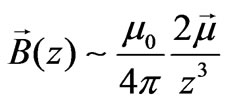 (3)
(3) (4)
(4)
 ]
]
 Dashing[{0.02}]}, PlotRange->{All,{10,120}}];
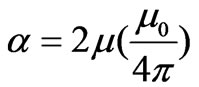 . The units of
  is Gauss.cm3, and when
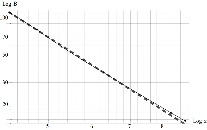
 (5)
(5)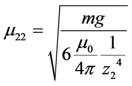 (6)
(6)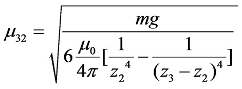 and
and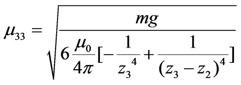 (7)
(7) and
and  are the solutions of the
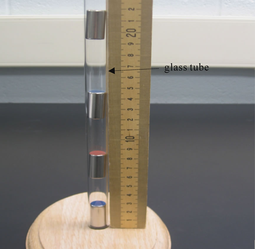
 are interpreted as the 2nd magnet of a three-magnet tower. Note that for the number of conducive equations, the value of m’s are one less than the number of the magnets. In our study we extend the static method from a minimum of a two-magnet tower to a five-magnet assembly. We provide one of the four equations for the five-magnet assembly,
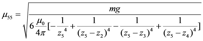 (8)
(8)

 at the instance when the bouncing magnet is accelerating upward along the z-axis yields,
 (9)
(9) /m is the viscous coefficient per mass. We utilize the mean value of the measured magnetic dipole moment according to the procedures discussed in Subsections 3.1 and 3.2. Therefore, with the exception of g all of the coefficients of Equation (9) are known. For a set of appropriately chosen initial conditions, namely the initial height of the freely dropped magnet we apply NDSolve and solve Equation (9) numerically. With trial and error we search for g such that the solution of Equation (9) reasonably duplicates the data. Figure 7 displays the solution of Equation (9) for g=1.9. Utilizing the magnet mass the coefficient of the viscous force, G yields 0.0437 kg.s-1. According to the data shown in Figure 5 we had anticipated a small value for G such as the one we deduced from our theoretical model. To run our code we supply the known parameters in MKS units.
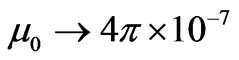 ,
, , meanm®3.63, g ®1.9};
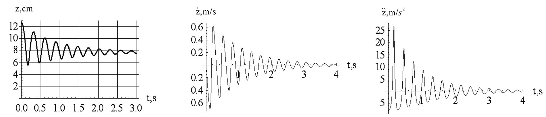
 ,m/s"},PlotRange®All,PlotStyle®{Black},AxesOrigin®{0,0}];
 m/s2"},PlotRange®All,AxesOrigin®{0,0},PlotStyle®{Black}];
 ,
, , and
, and  implicitly. We also plot one three-dimensional set,
 . With the exception of the velocity vs. position graph,
  , commonly known as the phase diagram, the other three graphs as shown in Figure 9 are innovative and fresh.
 ,4m/s"},PlotRange®All,PlotStyle®{Black}];
 ,10-1m/s2"},PlotRange®All,PlotStyle®{Black},AspectRatio®1.2];
 ,5m/s","
 ,10-1m/s2"},PlotRange®All,PlotStyle®{Black}];
 ,5m/s","
 ,10-1m/s2"},BoxRatios®1,PlotStyle®{Thickness[0.007],Black},PlotPoints®120];
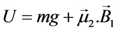 . Applying Equation (3) the potential energy for a pair of identical magnets yields,
 . Now, we utilize the solution of Equation (9) and evaluate the time-dependent values of the kinetic and potential energies. A display of the total energy vs. time is shown on the left panel of Figure 10. On the right panel of the same figure we display the rate of loss of energy, d/dt E(t); the loss of energy is associated with the viscous force.