Int'l J. of Communications, Network and System Sciences
Vol.6 No.4(2013), Article ID:29843,12 pages DOI:10.4236/ijcns.2013.64019
Reliability Analysis of Controller Area Network Based Systems—A Review
1School of Electronics Engineering, VIT University, Vellore, India
2Department of Electrical Engineering, Indian Institute of Science (IISc), Bangalore, India
Email: gerardine@vit.ac.in, zachariahcalex@vit.ac.in, lawrn@ee.iisc.ernet.in
Copyright © 2013 Gerardine Immaculate Mary et al. This is an open access article distributed under the Creative Commons Attribution License, which permits unrestricted use, distribution, and reproduction in any medium, provided the original work is properly cited.
Received January 28, 2013; revised February 28, 2013; accepted March 18, 2013
Keywords: Reliability Analysis of Controller Area Network Based Systems; Fault-Tolerant CAN Based Systems
ABSTRACT
This paper reviews the research work done on the Reliability Analysis of Controller Area Network (CAN) based systems. During the last couple of decades, real-time researchers have extended schedulability analysis to a mature technique which for nontrivial systems can be used to determine whether a set of tasks executing on a single CPU or in a distributed system will meet their deadlines or not [1-3]. The main focus of the real-time research community is on hard real-time systems, and the essence of analyzing such systems is to investigate if deadlines are met in a worst case scenario. Whether this worst case actually will occur during execution, or if it is likely to occur, is not normally considered. Reliability modeling, on the other hand, involves study of fault models, characterization of distribution functions of faults and development of methods and tools for composing these distributions and models in estimating an overall reliability figure for the system [4]. This paper presents the research work done on reliability analysis developed with a focus on Controller-Area-Network-based automotive systems.
1. Introduction
Scheduling work in real-time systems is traditionally dominated by the notion of absolute guarantee. The load on a system is assumed to be bounded, and known, worstcase conditions are presumed to be encountered, and static analysis is used to determine that all timing constraints (deadlines) are met in all circumstances. This deterministic framework has been very successful in providing a solid engineering foundation for the development of real-time systems in a wide range of applications from avionics to consumer electronics. However, the limitations of this approach are now beginning to pose serious research challenges for those working in scheduling analysis. A move from a deterministic to a probabilistic framework is advocated in [5].
When performing schedulability analysis (or any other type of formal analysis) it is important to keep in mind that the analysis is only valid under some specific model assumptions, typically under some assumed “normal condition,” e.g., no hardware failures and a “friendly” environment. The “abnormal” situations are typically catered for in reliability analysis, where probabilities for failing hardware and environmental interference are combined into a system reliability measure. This separation of deterministic (0/1) schedulability analysis and stochastic reliability analysis is a natural simplification of the total analysis, which unfortunately is quite pessimistic, since it assumes that the “abnormal” is equivalent to failure; in particular, for transient errors/failures, this may not at all be the case. Thus, even in cases where the worst case analysis deems the system to be unschedulable, it may be proven to satisfy its timing requirements with a sufficiently high probability [4]. The basic argument of the work in [4] is that for any system (even the most safety critical one) the analysis is valid only as long as the underlying assumptions hold. A system can only be guaranteed up to some level, after which we must resort to reliability analysis. The main contribution of [4] is in providing a methodology to calculate such an estimate by way of integrating schedulability and reliability analysis. Furthermore, this type of reasoning is especially pertinent considering the growing trend of using wireless networks in factory automation and elsewhere. The error behavior of such systems will most likely require reliability to be incorporated into the analysis of timing guarantees. The ability to tolerate faults becomes a more critical characteristic for hard real-time systems, in which the missing of deadlines can have catastrophic results.
Systems with requirements of reliability are traditionally built with some level of replication or redundancy so as to maintain the properties of correctness and timeliness even in the case of faults. Faults can be tolerated by using hardware, software, information and time redundancy. In certain classes of applications, it may not be feasible to provide hardware redundancy due to space, weight and cost considerations. Such systems need to exploit software, information and time redundancy techniques and especially the combination of these techniques. However, the implementation of such systems increases the complexity of keeping the system computation in compliance with the requirements specification. Effective schedulability analysis, which takes the fault model, fault tolerance mechanisms and the scheduling algorithm into consideration, is needed to guarantee the timeliness property [6]. A central feature of these systems is that the behavior is periodic, with a hyperperiod that is equal to the LCM of the periods of the constituent tasks. Section 2 presents the related research work. Section 3 presents an introduction to Reliability modeling and Section 4 presents the general real-time system model, the fault-tolerant communication model and the applied reliability metrics.
2. Related Work
Formal analysis approaches of fault-tolerant real-time systems have been addressed by some previous research activities. In [7], Burns presents a method to explore tasks for the probability of missing their deadline. Broster proposes an extension of this method to derive probabilistic distribution functions of response times on a CAN bus [8]. The author assumes non-preemptive transmission behavior. De Lima introduces an approach to calculate an optimal priority assignment for recovery mechanisms, leading to a minimum deadline miss probability [9]. However, the approaches [7-9] have certain limitations, leading to extremely pessimistic results. This pessimism is mainly due to two basic assumptions. First of all only the worst-case is considered, i.e. that situation in which each task has the highest deadline failure probability (DFP). Furthermore, on the error penalty is generally overestimated due to the assumption that each error affects that task with the maximum runtime, leading to maximum reexecution/retransmission overhead. A detailed discussion of these limitations has been presented in [10]. In [11], the authors propose another method that is not restricted to pure worst-case analysis. Instead they consider a priority-driven CAN bus during a period of time, and include individual response time analysis for each message. However, it is still assumed that each error causes the maximum overhead. Another issue is that the error model is assumed to be deterministic, being simply specified by a minimum distance between two consecutive errors. Consequently no derivation of reliability is feasible. Instead it is only possible to decide whether the system is working or not under the given assumptions, without any measure to characterize the degree of safety. In [12], the deterministic error model is presented as a generalization of the relatively simplistic error model by Tindell and Burns [13]. The error model specifically addresses the following:
• Multiple sources of errors: Handling of each source separately is not sufficient; instead, they have to be composed into a worst case interference with respect to the latency on the bus.
• Signaling pattern of individual sources: Each source can typically be characterized by a pattern of shorter or longer bursts, during which the bus is unavailable, i.e., no signaling will be possible on the bus. This model is, just as Tindell and Burns’ model, deterministic in that it models specific fixed patterns of interference. Section 3 presents general reliability modeling for such distributed real-time systems, as presented in [4].
An alternative is to use a stochastic model with interference distributions. Such a model is proposed by Navet et al. [14], who uses a Generalized Poisson Process to model the frequency of interference, as well as their duration (single errors and error bursts). In close association to this stochastic approach, Section 4 presents a general real time system model according to [15] and Section 5 presents a formal analysis methodology using the stochastic approach as presented in [15].
A study done by Burns, Davis and Punnekkat [16], provides schedulability tests for fault tolerant task sets scheduled with the full preemptive priority algorithm. The recovery of tasks is modeled as alternative tasks that should be executed to recover the system from an erroneous state. The authors have shown that fault-tolerance based on error-recovery techniques can be easily modeled by response time analysis. The response time analysis of [1] is extended to implement this fault tolerance approach. Fixed point recursive computations are used to determine the response time of each task if a fault occurs during its execution. Based on the work of [16], Lima and Burns [17], also studied the approach to run the recovery of tasks with higher priorities, and provided an effective schedulability test to guarantee the predictability of a system with this character. The methods used in [16,17] assume a full preemptive priority scheduling model. In [6], group-based preemptive scheduling is considered. In this scheme, tasks can be put into groups. Within a group, tasks behave like non-preemptable tasks, i.e. they are not allowed to be preempted by tasks with higher priorities in the same group. For tasks with a priority higher than the highest priority within the group, all the tasks within the group can be preempted by them. Besides providing the flexibility of mixing preemptive and non-preemptive scheduling, the group-based preemptive scheduling also provides a means to control resource access. Within a group, tasks execute serially, and there is no conflict of access to the shared resource. One can define inter-task invariants on the shared state and be assured that, while the present task is running, no other tasks can violate the invariants. The group-based preemptive scheduling provides a flexible mechanism to define the preemptive relations between tasks. However, this scheduling scheme together with a resource access synchronization protocol and requirements of fault tolerance makes the predication of real-time system’s behavior more difficult than traditional scheduling schemes. The major contribution of the work is an algorithm to calculate the worst-case response time for tasks under the fault-tolerant group-based preemptive scheduling.
In [18], mixed critically applications are addressed, and the native CAN fault-tolerant mechanism assumes that all messages transmitted on the bus are equally critical, which has an adverse impact on the message latencies, results in the inability to meet user defined reliability requirements, and, in some cases even leads to violation of timing requirements. As the network potentially needs to cater to messages of multiple criticality levels (and hence varied redundancy requirements), scheduling them in an efficient fault-tolerant manner becomes an important research issue. In [18], the authors present a methodology which enables the provision of appropriate guarantees in CAN scheduling of messages with mixed criticalities. Their approach involves definition of fault tolerant feasibility windows of execution for critical messages, and off-line derivation of optimal message priorities that fulfill the user specified level of fault-tolerance. To enhance the dependability of CAN communication, research on the on-line fault diagnosis is carried out in [19], a monitor is designed to diagnose faults in CAN nodes and a hybrid method with active and passive mode is presented to diagnose faults among communication links.
3. Reliability Modeling with Deterministic Error Model
Reliability is defined as the probability that a system can perform its intended function, under given conditions, for a given time interval. In the context of an automobile, its intended function is to provide reliable and cost-effective transport of men and material. At a subsystem level, such as for an Antilock Braking System (ABS), this boils down to performing the tasks (mainly input_sensors, compute_control, and output_actuators, etc.,) as per the specifications. Being part of a real-time system, the specifications for ABS imply the necessity for the results to be both functionally correct and within timing specifications [4].
A major issue here is how to compose hardware reliability, software reliability, environment model, and timing correctness to arrive at reasonable estimates of overall system reliability. A central feature of these systems is that the behavior is periodic, with a hyperperiod that is equal to the LCM of the periods of the constituent tasks.
The following probabilities are defined


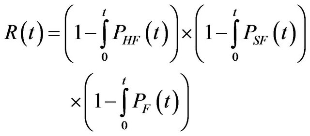
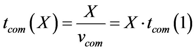
The reliability of the system is the probability that the system performs all its intended functions correctly for a period. This is given by the product of cumulative probabilities that there are no failures in hardware, software, and communication subsystem during the period. That is,
 (1)
(1)
In [4], only on the final term in (1) is concentrated, i.e., the probability that no errors occur in the communication subsystem. They do not concentrate the faults in the hardware or in the software of such a system. Instead, it is looked at from a system level and one treats its correctness as the probability of correct and timely delivery of message sets. Since the main cause for an incorrect (corrupted, missing, or delayed) message delivery is environmental interference, an appropriate modeling of such factors in the context of the environment in which the system will operate is essential for performing reliability analysis. A completely accurate modeling of the probability of timely delivery of messages is far from trivial and hence certain simplifying assumptions are made in order to divide the problem into manageable portions [4].
A. Reliability Estimation By definition, reliability is specified over a mission time. Normally, a repetitive pattern of messages (over the least common multiple (LCM) of the individual message periods) is assumed. Each LCM (hyperperiod) is typically a very small fraction of the mission time.
Let t represents an arbitrary time point when the external interference hits the bus and causes an error. If one can assume zero error latency and instantaneous error detection, then t becomes the time point of detection of an error in the bus due to external interference.
The following probabilities are defined:
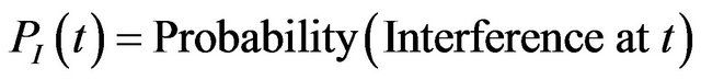


By relying on the extensive error detection and handling features available in the CAN, one can safely assume that an error in a message is either detected and corrected by retransmission, or will ultimately result in a timing error. This allows to ignore PC(t), and define in this context the probability of communication failure due to an interference starting at t as
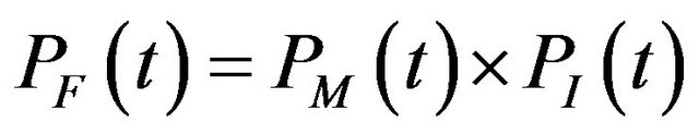 (2)
(2)
In the environment model in [12], the authors have assumed the possibility of an interference I1, having a certain pattern, hitting the message transmission. Let  be the probability of such an event occurring at time t. It is also assume that another interference I2, having a different pattern, can hit the system at time t with a specified probability, for example,
 . In [12], the authors assumed that both cases of interference hit the message transmission in a worst case manner, and looked at their impact on the schedulability.
In [4], the realism is increased by relaxing the requirement on the worst case phasing between schedule and interference. It should be noted that there is an implicit assumption that these cases of interference are independent.
B. Failure Semantics In the above presentation, it is assumed that a single deadline miss causes a failure. This may be true for many systems, but in general, the failure semantics do not have to be restricted to this simple case. For instance, most control engineers would require the system to be more robust, i.e., the system should not loose stability if single deadlines, or even multiple deadlines, are missed. Tolerable failure semantics for such a system [4] could for instance be: “three consecutive deadlines missed, or five out of 50 deadlines missed.” Such a definition of failure is more realistic and also leads to a substantial increase in reliability estimates, as compared to the single deadline miss case. To simplify the presentation, the authors in [4] stick to the simple “single missed deadline” failure semantics for the time being; however, it is noted that systems that fail due to a single deadline miss should be avoided, since they are extremely sensitive.
In particular, for critical systems, the designer has an obligation to make the system more robust. For instance, for a simple system a more reasonable failure semantics would be: “a failure occurs if more than two out of ten deadlines are missed.”
It should be noted that changing the failure semantics may have implications for the design, since it is to be made sure that the system appropriately can handle the new situation, for example, in this case, that a few deadline misses can be tolerated.
C. Calculating Failure Probabilities To calculate the subsystem reliability, first one needs to calculate the failure probability (in this case of the communication subsystem subject to possible external interference), i.e., the probability of at least one failure (defined as a missed deadline) during the mission time. In doing this, it is assumed that the interference-freesystem is schedulable, i.e., that it meets all deadlines with probability 1. Due to the bit-wise behavior of the CAN bus, and with respect to the external interference, a discretization of the time scale is made, with the time unit corresponding to a single bit time τbit (1 s for a 1-Mb/s bus), i.e., no distinction is made between an interference hitting the entire bit or only a fraction of it. In either case, the corruption will both occur and be detected [4].
Two types of interference sources are considered in [4].
• Intermittent sources, which are bursty sources that interfere during the entire mission time T, and are for an interference source I characterized by a period TI and a burst length lI (where lI < TI )• Transient sources, which are bursty sources of limited duration. These occur at most once during a mission time T, and for an interference source J are characterized by a period TJ, a burst length lJ, and a number of bursts nJ (where lJ < TJ and ), For a single intermittent source I, the probability of a communication failure during the mission time is defined as follows:
 (3)
(3)
where  denotes the conditional probability of a communication failure, given that the system was hit by interference from source I at time t, denoted by
 . Since interference and bus communication are independent, it follows that
 .
.
 is calculated by simulation, i.e., the bus traffic during a mission is simulated, including the effects of interference, to determine if any communication failure (deadline violation) occurs. This will for each result in either 0, if no deadline is missed, or 1, if a deadline miss is detected.
For a single transient source J, the probability of a communication failure during the mission time is defined as follows:
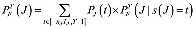 (4)
(4)
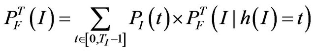
where PJ(t) denotes the probability that the first transient interference hits the system at time t, and  denotes the conditional probability of a communication failure during T due to interference from J, given that the interference J starts at time t. In the above summation, all possible full or partial interference from the transient source during mission time are considered. The interval
  specifically captures initial partial interference, starting before mission time, but ending during mission. Since interference and bus communication are independent, it follows that
 .
.
 is calculated by simulation, just as above.
The number of scenarios to simulate here is potentially much larger than for an intermittent source, since typically . However, the number of simulations can be reduced, since the probability of failure is independent of the hyperperiod (LCM of individual message periods), in which the interference hits the system. It can be proved that
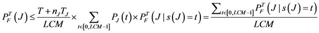 (5)
(5)
It should be noted that a slight pessimism is introduced (which is the reason for the ≤) since the probability for failure in T is lower toward the end, when the interference bursts are extending past the end of T. However, since it is assumed that , the introduced pessimism can be considered negligible.
Also, it is to be noted that in (5) the effects of the interference starting before the LCM is covered by the interference on the subsequent LCM, which is the reason for starting the summation with t = 0 [rather than 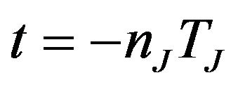 as in (4)]. Finally, it is noted that by not counting the interference starting outside the very first LCM (at the beginning of the mission time), some optimism is introduced, but since the assumption of
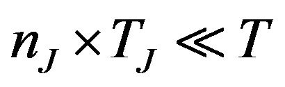 this optimism is insignificant.
To be more precise, a fraction of (4),
![]()
could be added to (5) in order to cover for the pre-mission time-triggered transient faults.
The above basic analysis is now extended to the analysis of multiple sources of interference. First, the presence of two independent sources of interference is considered. There are totally three cases to consider, namely 1) Two intermittent sources I1 and I2
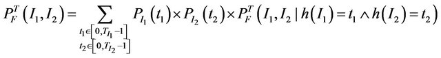 (6)
(6)
2) Two transient sources J1and J2
 (7)
(7)
3) One intermittent and one transient source
 (8)
(8)
The number of scenarios to simulate for the above three cases are in the order of , T2, and
 , respectively. This may be rather large, especially for the last two cases. By observing symmetries in the formulas, however, the number of scenarios can be reduced. For case 3), consider the following two mutually exclusive situations: 1) LCM ≥ TI1, which leads to the following reduced formula:
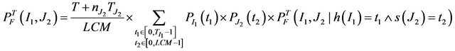 (9)
(9)
and 2)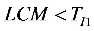 , which leads to the following reduced formula:
 (10)
(10)
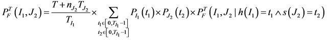
The above two equations can be combined into
 (11)
(11)
and, thus, the number of scenarios is reduced from the order of TI1 × T to the order of TI1 × max (LCM, TI1).
Finally, the general formula for an arbitrary number of interference sources of either type (n intermittent and m transient sources of interference) is presented as [4]
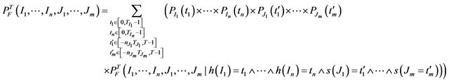 (12)
(12)
D. Approach to Analysis The above equations define the probability of communication failure given a set of sources interfering with the communication according to specified patterns [4]. In the modeling, they additionally specify the probability that an interference source actually is active during the mission. This gives the following:
• One has a set K of external sources of interference, where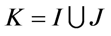 , I is a set of intermittent sources of interference and J is a set of transient sources, as defined above.
• Each interference source  is either active or inactive during a mission. The probability for each source to be active is
 , and the probability for inactivity is consequently
 .
.
For a scenario with a single intermittent interference source I1 and a single transient interference source J2, we can now (with a slight generalization of the notation) define the probability of a communication failure in a mission as follows:
 (13)
(13)
which for an arbitrary set I of intermittent sources and an arbitrary set J of transient interference sources can be generalized to
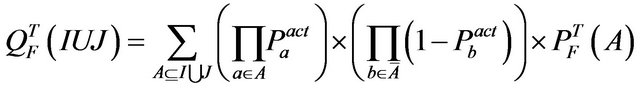 (14)
(14)
where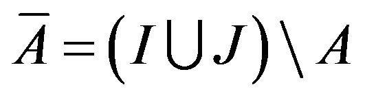 . Intuitively, (14) defines the failure probability for a system that is potentially subjected to interference from a set
  of interference sources as the sum of the weighted probabilities that a failure occurs in each of the possible combination of sources.
4. Reliability Modeling with Fault Tolerant Communication Model
This section presents an introduction to the general real-time system model, the fault-tolerant communication model and the applied reliability metrics, as presented in [15].
A. General System Model The calculation of reliability is illustrated based on a system bus that connects the processing nodes in an embedded system. On each processing node a certain number of processes is executed. Whenever two processes on different nodes need to communicate, a message is sent over the bus. For that purpose, a logical communication channel will be assigned to each pair of communicating processes. An example system with three logical communication channels τl, τ2 and τ3. (as shown in Figure 1) is considered. This is a simple system, but it is sufficient to present and demonstrate the analysis methodology.
Tasks are coupled by event streams to indicate dependencies between them. An event stream is defined as a numerical representation of the timing of event occurrences [15]. Whenever an event occurs at a task’s input, this task is activated and has to either execute a program or to transmit data. Event streams can be specified by
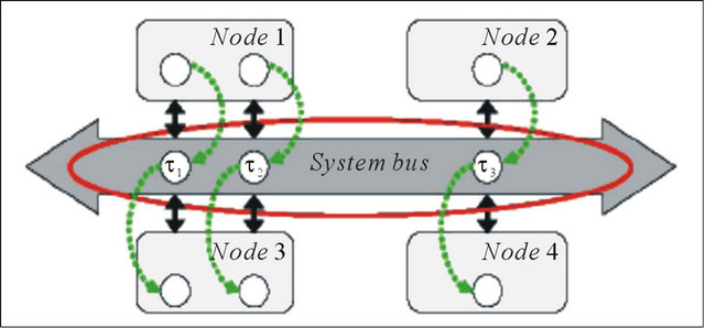
Figure 1. System model.
several characteristic functions. The upper-bound arrival function  describes the maximum number of events at τi’s input during an interval of length t. In [15], the authors restrict their consideration to strictly periodic activations of the channels τl, τ2 and τ3, with periods T1, T2 and T3 respectively and without any release jitter. This is a reasonable assumption for a wide variety of applications, e.g. signal processing or control loops. Further on perfectly synchronized clocks on each node are assumed.
Each message has a deadline that is equal to the period of the corresponding channel. Due to the fact that multiple channels may concurrently request access to the bus, a scheduler is adopted to decide which channel bus will be granted access in case of conflicts.
The scheduling policy is static-priority non-preemptive, i.e. only the channel with the highest priority may transmit data. Preemptions of running transmissions are not permitted. This communication model corresponds to the CAN bus.
B. Fault-Tolerant Communication Model In this work, a single bus is assumed as communication medium. That is a very frequently used medium, both on chip and in distributed applications, such as in automotive electronics. In contrast to processes running on a CPU, the workload of a communication channel is often measured by the amount of data X to be transmitted within one job. Given the transmission speed Vcom, it is possible to compute the effective time tcom (X) a message of size X (in bits) utilizes the bus (without any fault tolerance measures):
 (15)
(15)
For the sake of clarity, all the messages of a communication channel τi are assumed to have the same length Xi. However the proposed method is also well-suited for channels with messages of different lengths. In this case it would be necessary to know the sequence of transmitted data (and thus the sequence of message lengths) a priori (e.g. MPEG). For scheduling analysis it is essential to know tcom instead of the amount of data. However the probabilistic considerations are based on the measure of bit error rate (BER), i.e. the relative amount of erroneous bits during transmission. As a consequence, the value of X is relevant to determine the probability that a message suffers from a certain number of bit errors. It should be noted that only independent errors are considered. Burst errors which might corrupt consecutive bits beyond message boundaries are excluded by this restriction. This is a reasonable assumption for on-chip buses [15]. Otherwise the effect of burst errors can be turned into the effect of single errors by determining a maximum burst length and assuring that each burst may corrupt at most one message. For this purpose a protection time has to be defined that specifies an interval between messages where bus access is not allowed.
There exists a wide variety of fault tolerance techniques to protect data transmission, commonly classified into error detecting codes (EDC) and error correcting codes (ECC) [15]. EDCs append some redundancy bits to the message which enable the receiver to detect whether an error has occurred. If an error is detected, a retransmission of the message is necessary to avoid a functional failure. However in real-time systems this may lead to timing failures due to missed deadlines. In [15] the focus is on the analysis of EDC-protected communication. Each job can have an arbitrary number of transmission trials due to errors, as long as no deadline is missed. It is assumed that the number of redundant bits is message independent, as it is the case for many commonly used mechanisms, e.g. cyclic redundancy codes.
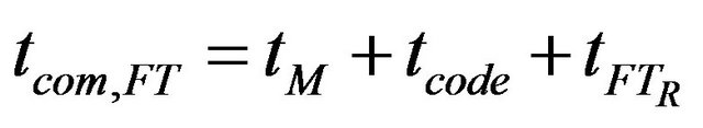
Figure 2 illustrates the EDC-related communication timing model for a single message. In addition to the sending and the receiving node and the communication medium, a fault tolerance layer is introduced to realize the protection against transmission errors. In general the effective transmission time can be calculated as follows:
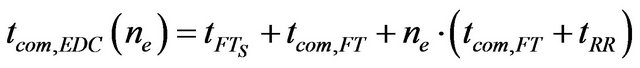 (16)
(16)
where tFTS is the computation time for redundancy bits tcom,FT is the time of a single transmission trial using a fault tolerant bus tRR is the transmission time for the retransmission request ne is the number of erroneous transmission trials tcom,FT is composed of the transmission times tM for the message payload and tcode for the redundant bits and the time tFTR wasted for evaluation of the redundant bits:
 (17)
(17)
Corresponding to the discussion in [9] different strategies can be applied to schedule retransmissions in a static-priority based scheduling scheme. In [15] two simple strategies are adopted:
Normal Priority Retransmission: Retransmissions have the same priority as the original transmission.
Highest Priority Retransmission: Retransmissions
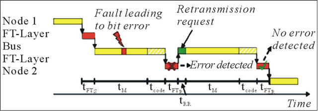
Figure 2. EDC communication model.
always have the highest priority.
C. Reliability Model The lifetime of a system is modelled with a random variable L that represents the time the system is running without failure. FL depicts the distribution function of L. In [15] the commonly used notion of reliability R as metric is adopted, which is defined as the complementary function of FL:
 (18)
(18)
Practically R(t) denotes the probability that within an interval [0, t] no failure occurs [15].
5. Reliability Analysis Methodology with Probabilistic Error Model
This analytical method is aimed to overcome the limitations discussed in Section 2. For this purpose, a job-wise analysis is introduced, i.e. the number of tolerable errors is considered w.r.t. the job’s actual interference situation. Furthermore the probability that this number is not exceeded will be calculated for each transmission job separately. This procedure has to be performed for all jobs within the hyperperiod of the bus. After one hyperperiod has been completed, channel activations and load situation are repeated in exactly the same way as before. Consequently all probabilistic information which are necessary to derive a reliability function are already included into one hyperperiod [15].
The fact that the job τi,j meets its deadline will be referred to with Si,j (success of τi,j).
The probability that the job τi,j meets its deadline is denoted with P[Si,j].
The probability of Si,j provided that some jobs  have already met their deadlines is denoted as conditional probability with
The set of all jobs τi,j that have been activated in the interval [0, t] is denoted with J(t),and the cardinal number| J(t)| with M:
 (19)
(19)
Consider a time interval [0, t] and a list J(t) as defined by Equation (19). Furthermore J(t) is sorted by the monotonically increasing activation times of the jobs, with ties broken such that the jobs of higher priority tasks are considered before those of lower priority tasks. Based on this notation, reliability R(t) can be defined as the probability that all jobs in J(t) meet their deadlines, i.e.:
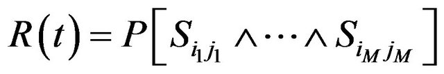 (20)
(20)
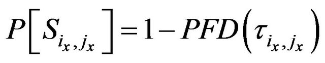
Consider that single success probabilities represent the probabilistic complements of the individual probabilities of failure on demand for each job, i.e.
 Equation (19) can be converted using the laws of probabilities:
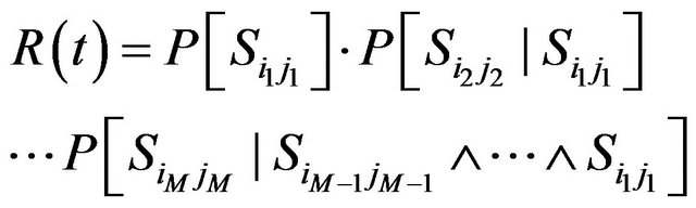 (21)
(21)
Hence computation of these conditional probabilities remains as the central challenge. This problem can be divided into determining the maximum number of tolerable errors per job and computing the probability that this number will not be exceeded. Before going into details, some reflections concerning the analysis interval are presented.
A. Analysis Interval Equation (20) represents the basic analysis methodology of jobwise success probability calculation. As explained at the begining of this section the job-wise analysis has to be performed for exactly one hyperperiod, which is equal to . If the reliability for one hyperperiod in known, reliability for A hyperperiods can be extrapolated by raising
  to the power of A:
 (22)
(22)
Hence even if R(t) for large values of t is considered the analysis complexity is the same.
B. Number of Tolerable Errors An algorithm to compute the maximum number of tolerable errors per job is now presented. For the sake of clarity, the overhead in expressions tRR and tFTs is ignored. Thus a message that has to be retransmitted ne times has an overall transmission time of . Further on the more compact notation jx is introduced to refer to a certain job
  ∊ J(t).
Figure 3 demonstrates a simple scenario consisting of two jobs jc‒1 and jc, with jc‒1 having higher priority than jc. Job jc is the considered job that should be evaluated for the maximum number of tolerable errors.
In the example, there exist several combinations of retransmissions of jc‒1 and jc without jc missing its deadline, as shown in Table 1. In contrast, using the existing
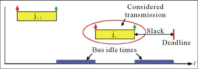
Figure 3. Transmission scenario.
Table 1. Tolerable retransmissions.
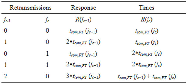
approach of exclusively considering the worst-case situation, i.e. that scenario when jc‒1 and jc are activated simultaneously, would indicate no tolerable error at all.
Figure 4 illustrates the method to compute all tolerable retransmissions for the considered job jc algorithmically. It again refers to the example from Figure 3. In general the objective is to determine the number of erroneous transmissions the currently considered job jc is able to tolerate, including transmission errors in jobs other than jc which cause a certain delay to jc due to scheduling effects [15].
In Figure 4, each node represents a dedicated error scenario sc,k. 1t is labeled with the corresponding error vector e-c,k. An edge represents an error event 
 to denote that the last transmission trial of job jc-x is disturbed by an error.
The fact that an arbitrary error scenario Si,k of a job ji actually occurs is denoted with ωi,k.
A response time analysis is performed to determine whether the considered job jc will meet its deadline under the actual interference situation and the error scenario represented by the node. If jc meets its deadline, all successors of the node that represents the currently considered error scenario within the tree will be explored. Otherwise the node is tagged as not working, what implies that all its successors are not working too. From the graph-theoretic point of view a non-cyclic directed graph (i.e. a tree) is traversed using a depth first search, where nodes tagged as not working are used as an abort criterion. The search terminates when there are no remaining working nodes with unexplored successors, i.e. when all leaves are tagged as not working. At this point, the working set  of the job jc is found. It is separated from the non-working set by the working front
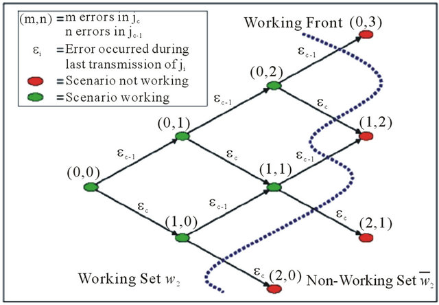
Figure 4. Error scenario tree.
as depicted in Figure 4.
Theoretically, jc’s completion may be delayed by all other jobs  that have been activated beforehand. This would lead to a growing dimension of the error vector from job to job and thus to a depth explosion of the search tree. To avoid this problem, only the last D jobs which have been activated before jc are included into the tree-based analysis. The parameter D is called the search depth. A bounded search depth assures a constant dimension of the error vector. This strategy may cause a disregard of certain error scenarios which generate a failure. Hence an overestimation of reliability may occur, leading to a non-strictly conservative analysis approach. However the experiments in [15] show a significant accordance with the simulation results, demonstrating the accuracy of this technique for reliability estimation and its practicability for system evaluation even with bounded search depth. The value of D is adjustable, depending on the demands on accuracy and computational complexity. Multiple analysis runs with increasing D-values have to be performed until the result variation between two analyses falls below a specified threshold.
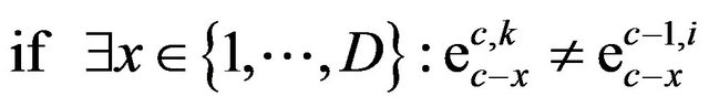
C. Success Probability Computation Reconsidering the two steps mentioned above, the remaining problem is the calculation of the conditional success probabilities. That is considering a job jc, expression (23) has to be evaluated.
 (23)
(23)
Because the occurrences  of all scenarios in wc are mutually exclusive, the overall probability that exactly one of these scenarios actually appears can be computed by summing up the individual probabilities:
![]() (24)
(24)
It is shown in [15] that Equation (24) can be evaluated for a given bit error rate BER and known message lengths Xc.
In this context the following abbreviations are introduced to proceed with a more compact notation:
 (25)
(25)
Consequently, Equation (24) is simplified
 (26)
(26)
Equation (26) is rearranged corresponding to the law of total probability:
 (27)
(27)
Thus the following case differentiation is used:
1) 
2) 
 (28)
(28)
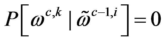
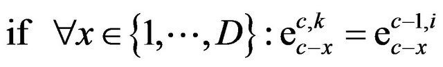
Then the probability 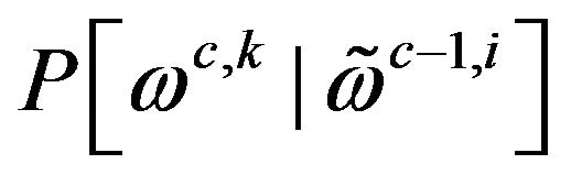 can be computed according to Equation (29).
 (29)
(29)
where
 is P[Transmission erroneous]
 is P[Transmission correct]
 is P[
is P[ erroneous transmissions]
Thus it is shown in that Equation (24) can be evaluated for a given bit error rate BER and known message lengths Xc.
6. Conclusions
Research on schedulability analysis for fixed priority scheduling can be split to two classes. One class of techniques is based on utilization bound U, which allows a simple test of the form ΣUi ≤ U to determine a task set’s schedulability [6]. For example, in Rate-Monotonic Scheduling (RMS), U = n(21/n − 1), where n is the total number of tasks. These methods have low overheads and adapt to online schedulability test. Their shortcoming is their pessimism, since some schedulable task sets may have higher utilizations than the bound U. The other class of techniques is based on the response time analysis techniques, which can provide exact schedulability analysis [1,16,17]. Such techniques have been increasingly developed for less restrictive computational models, thus allowing tasks to interact via shared resources, to have deadlines less than their periods [1], release jitter [1] and deadlines greater than their periods [6]. Furthermore, these methods can also be used in distributed real-time systems [6]. Compared with the methods based on utilization bound, response time analysis has higher overhead, so it is usually used as an off-line test.
The developed notion of a probabilistic assessment of schedulability has been supported [5] and shown how it can be derived from the stochastic behaviour of the work that the real-time system must accomplish [5]. Modelling faults as stochastic events means that an absolute guarantee cannot be given. There is a finite probability of some specified number of faults occurring within the deadline of a task. It follows that the guarantee must have a confidence level assigned to it and this is most naturally expressed as a probability. One way of doing this is to calculate the worst case fault behaviour that can (just) be tolerated by the system, and then use the system fault model to assign a probability to that behavior [4].
A method that allows controlled relaxation of the timing requirements of safety-critical hard real-time systems is presented [4]. The underlying rational is that no real system is (or can ever be) hard real time, since the behavior of neither the design nor the hardware components can be completely guaranteed. By integrating hard real-time schedulability with the reliability analysis normally used to estimate the imperfection of reality, we obtain a more accurate reliability analysis framework with a high potential for providing solid arguments for making design tradeoffs, e.g., that allow a designer to choose a slower (and less expensive) bus or CPU, even though the timing requirements are violated in some rare worst case scenario.
Using traditional schedulability analysis techniques, the designer will in many cases have no other choice than to redesign the system (in hardware, software or both). However, by resorting to the approach in [4], it is seen that the probability of an extreme error situation arising is very low and thus the designer may not need to perform a costly redesign.
It is well known [4] that a control system that fails due to a single deadline miss is not robust enough to be of much practical use. Rather, the system should tolerate single deadline misses, or even multiple deadline misses or more complex requirements on the acceptable pattern of deadline misses. These requirements should of course be derived from the requirements on stability in the control of the external process. The possibility to handle such requirements in the analysis can makes the use of the resources even more efficient, i.e., a tradeoff situation between algorithmic fault tolerance and resource usage is achieved. By considering each message separately, the reliability could be increased by incorporating algorithmic fault tolerance for functions which are dependent on a message that has the lowest reliability [4].
An algorithm to determine the maximum number of fault corrections and the corresponding probability of a missed deadline in case of periodic, priority driven communication systems during a period of time is presented [15].
An approach for the efficient fault-tolerant scheduling of messages of mixed criticality in CAN which provides guarantees for variable levels of redundancy for critical messages is presented [18]. This method guarantees the user a specified level of redundancy, as well as ensuring a short latency for non-critical messages. The concepts that have been introduced are that of a fault-tolerant window for critical messages, and fault-aware windows for non-critical messages, thus providing a variable level of redundancy requirement per message.
A comprehensive method to diagnose CAN nodes and communication links faults is presented [19]. The method uses a passive and active diagnosis approach which can be efficiently implemented and applied to a CAN system providing on-line fault diagnosis.
The method in [4] could be extended in various directions, such as including stochastic modeling of external interference, distributions of transmission times due to bit stuffing, distributions of actual queuing times, distributions of queuing jitter, as well as applying the framework to CPU scheduling, including variations in execution times of tasks, jitter, periods for sporadic tasks, etc. Some of these extensions require dependency issues to be carefully considered. For instance, message queuing jitter may for all messages on the same node be dependent on interrupt frequencies. Assuming independence in such a situation may lead to highly inaccurate results. Another critical issue which should be given further attention is the sensitivity of the analysis to variations in model parameters and assumptions [4].
REFERENCES
- N. C. Audsley, A. Burns, M. F. Richardson, K. Tindell and A. J. Wellings, “Applying New Scheduling Theory to Static Priority Pre-Emptive Scheduling,” Software Engineering Journal, Vol. 8, No. 5, 1993, pp. 284-292. doi:10.1049/sej.1993.0034
- L. Sha, R. Rajkumar and J. P. Lehoczky, “Priority Inheritance Protocols: An Approach to Real-Time Synchronization,” IEEE Transactions on Computers, Vol. 39, No. 9, 1990, pp. 1175-1185. doi:10.1109/12.57058
- J. Xu and D. L. Parnas, “Priority Scheduling versus PreRun-Time Scheduling,” Real-Time Systems, Vol. 18, No. 1, 2000, pp. 7-23.
- H. Hansson, C. Norström and S. Punnekkat, “Integrating Reliability and Timing Analysis of CAN-Based Systems,” Proceedings of 2000 IEEE International Workshop Factory Communication Systems (WFCS’2000), Porto, 2000, pp. 165-172.
- A. Burns, G. Bernat and I. Broster, “A Probabilistic Framework for Schedulability Analysis,” Proceedings of the 3rd International Embedded Software Conference (EMSOFT03), Philadelphia, 13-15 October 2003, pp. 1- 15.
- L. Wang, Z. H. Wu and X. M. Wu, “Schedulability Analysis for Fault-Tolerant Group-Based Preemptive Scheduling,” Proceedings of the Reliability and Maintainability Symposium, Alexandria, 24-27 January 2005, pp. 71-76.
- I. Broster, G. Bernat and A. Burns, “Weakly Hard RealTime Constraints on Controller Area Network,” 14th Euromicro Conference on Real-Time Systems, Viena, 19-21 June 2002, pp. 134-141.
- I. Broster, A. Burns and G. Rodriguez-Navas, “Probabilistic Analysis of CAN with Faults,” 23rd IEEE Real-Time Systems Symposium, Austin, 3-5 December 2002, pp. 269- 278.
- G. M. de A. Lima and A. Burns, “An Optimal FixedPriority Assignment Algorithm for Supporting Fault-Tolerant Hard Real-Time Systems,” IEEE Transactions on Computers, Vol. 52, No. 10, 2003, pp. 1332-1346. doi:10.1109/TC.2003.1234530
- M. Sebastian and R. Ernst, “Modelling and Designing Reliable Onchip-Communication Devices in Mpsocs with Real-Time Requirements,” 13th IEEE International Conference on Emerging Technologies and Factory Automation, Hamburg, 15-18 September 2008, pp. 1465-1472.
- A. Burns, S. Punnekkat, L. Strigini and D. R. Wright, “Probabilistic Scheduling Guarantees for Fault-Tolerant Real-Time Systems,” Dependable Computing for Critical Applications, 1999, pp. 361-378.
- S. Punnekkat, H. Hansson and C. Norström, “Response Time Analysis under Errors for CAN,” Proceedings of IEEE Real-Time Technology and Applications Symposium (RTAS 2000), 2000, pp. 258-265.
- K. W. Tindell and A. Burns, “Guaranteed Message Latencies for Distributed Safety-Critical Hard Real-Time Control Networks,” Department of Computer Science, University of York, York, 1994.
- N. Navet, Y.-Q. Song and F. Simonot, “Worst-Case Deadline Failure Probability in Real-Time Applications Distributed over Controller Area Network,” Journal of Systems Architecture, Vol. 7, No. 46, 2000, pp. 607-617. doi:10.1016/S1383-7621(99)00016-8
- M. Sebastian and R. Ernst, “Reliability Analysis of Single Bus Communication with Real-Time Requirements,” Proceedings of the 2009 15th IEEE Pacific Rim International Symposium on Dependable Computing, 2009, pp. 3-10.
- A. Burns, R. Davis and S. Punnekkat, “Feasibility Analysis of Fault-Tolerant Real-time Task Set,” 8th Euromicro Workshop on Real-Time Systems, 1996, pp. 209-216.
- G. M. de A. Lima and A. Burns, “An Effective Schedulability Analysis for Fault-Tolerant Hard Real-Time Systems,” 13th Euromicro Conference on Real-Time Systems, 2001, pp. 209-216.
- H. Aysan, A. Thekkilakattil, R. Dobrin and S. Punnekkat, “Efficient Fault Tolerant Scheduling on Controller Area Network (CAN),” IEEE Conference on Emerging Technologies and Factory Automation (ETFA), Bilbao, 13-16 September 2010.
- H. S. Hu and G. H. Qin, “Online Fault Diagnosis for Controller Area Networks,” International Conference on Intelligent Computation Technology and Automation (ICICTA), Vol. 1, 2011, pp. 452-455.