Journal of Water Resource and Protection
Vol.5 No.2(2013), Article ID:27680,13 pages DOI:10.4236/jwarp.2013.52013
Using Artificial Neural Network to Estimate Sediment Load in Ungauged Catchments of the Tonle Sap River Basin, Cambodia
Interdisciplinary Graduate School of Medicine and Engineering, University of Yamanashi, Kofu, Japan
Email: heng_sokchhay@yahoo.com
Received November 30, 2012; revised December 30, 2012; accepted January 9, 2013
Keywords: Artificial Neural Network; Suspended Sediment Load; Ungauged Catchment; Lower Mekong Basin; Tonle Sap River Basin
ABSTRACT
Concern on alteration of sediment natural flow caused by developments of water resources system, has been addressed in many river basins around the world especially in developing and remote regions where sediment data are poorly gauged or ungauged. Since suspended sediment load (SSL) is predominant, the objectives of this research are to: 1) simulate monthly average SSL (SSLm) of four catchments using artificial neural network (ANN); 2) assess the application of the calibrated ANN (Cal-ANN) models in three ungauged catchment representatives (UCR) before using them to predict SSLm of three actual ungauged catchments (AUC) in the Tonle Sap River Basin; and 3) estimate annual SSL (SSLA) of each AUC for the case of with and without dam-reservoirs. The model performance for total load (SSLT) prediction is also investigated because it is important for dam-reservoir management. For model simulation, ANN yielded very satisfactory results with determination coefficient (R2) ranging from 0.81 to 0.94 in calibration stage and 0.63 to 0.87 in validation stage. The Cal-ANN models also perform well in UCRs with R2 ranging from 0.59 to 0.64. From the result of this study, one can estimate SSLm and SSLT of ungauged catchments with an accuracy of 0.61 in term of R2 and 34.06% in term of absolute percentage bias, respectively. SSLA of the AUCs was found between 159,281 and 723,580 t/year. In combination with Brune’s method, the impact of dam-reservoirs could reduce SSLA between 47% and 68%. This result is key information for sustainable development of such infrastructures.
1. Introduction
Rainfall and runoff, the main erosion agents, detach soil particles from its matrix and transport gravitationally the detached materials or sediments to surrounding rivers. In the rivers, sediments flow further downstream with streamflow. Suspended sediment load (SSL) is a major portion of the total load transported by streams [1] and commonly accounts for 85% to 95% [2]. Sediment has been becoming an important issue involving in sustainable development of water resources system. The Mekong2Rio conference also addressed the concern on food security which could be adversely affected by alteration of the sediment natural flow [3]. Construction of water storages (e.g. dam-reservoirs) can provide solutions to food security issues through increased irrigation and at the same time improve access to energy through hydropower generation. However, such developments could affect on fisheries through the loss of sediment trapped behind dam walls, for example. The Lower Mekong Basin (LMB) contains over 100 hydropower projects (HPP) and if there are no any effective countermeasures taken into account, their development could trap sediment around 26 Mt/year, 60% of the total basin production [4].
Quantification of sediment load is necessary not only during the project development stage but also along the course of operation until decommissioning [5-12]. It is interesting with regard to reservoir sedimentation, fish habitat, river utilization as well as biological sustainability in the whole river basin [13]. The most reliable way in estimating sediment load is the use of its observed records, but sediment sampling is very difficult and requires high experienced professionals because of its significant fluctuation within the river section [9] and userunfriendly measurement tools. Moreover, it is time consuming and costly [11,14]. These constraints have led to low frequency of sediment observation around the world and especially in developing and remote regions [1] such as the LMB. In response to this problem, modeling approach, based on different hydrological variables and terrain attributes, has been taken into consideration.
The unit stream power (USP) theory of Yang [15], the SHESED model of Wicks and Bathurst [16] and others known as the physically-based models, could be universally used to predict sediment yield of a watershed but it requires a lot of detailed information including hydrological, hydraulic and geological characteristics of the river basin, and as well as sediment characteristics itself. Preparation of such dataset will be difficult and costly. Furthermore, the stream power approach cannot predict well the SSL because, in rivers, the finest fraction of SSL is often a non-capacity load [17,18]. Similarly for process-based models such as the modified universal soil loss equation (MUSLE), introduced by Williams [19], and its family (USLE and RUSLE), they also require huge amount of input data. Data consumption and complex sediment transport mechanism have driven both physicallyand process-based models to be based on many simplifying assumptions and empirical relationships, particularly for rainfall and runoff erosive effects [7,20]. In consequence, their application in data scarce areas would yield high uncertain results or be completely infeasible.
Alternative approach to the processand physicallybased techniques is the utilization of data-driven models. Artificial neural network (ANN) is the most well-known and powerful data-driven method and it has been proved to be useful in modeling complex hydrologic processes or non-linear systems such as sediment transport [10,21, 22]. ANN forecasts outputs using experiences learned from historical data. This method is widely used because it does not require detailed information of the physical process controlling the system and generally applicable using available hydrological data. Tayfur [23] stated that ANN is a very practical and promising modeling tool for the study of sediment transport processes in data shortage regions. Kisi and Shiri [13] employed ANN to estimate daily suspended sediment concentration (SSC) in Eel River, California, and obtained a very satisfactory result with determination coefficient (R2) ranging between 0.82 and 0.95. In predicting daily SSL in Mississippi, Missouri and Rio Grande River in USA, Melesse et al. [11] found that ANN (0.65 ≤ R2 ≤ 0.96) for most cases is superior to other data-driven models: multiple linear/nonlinear regressions and autoregressive integrated moving average. In Longchuanjiang River, the Upper Yangtze Catchment in China, monthly SSL was modeled well by ANN with R2 varying from 0.66 to 0.89 in validation stage [24].
Singh et al. [12] compared two different models for predicting monthly SSL of Nagwa watershed in India and the results showed that ANN is better than MUSLE for larger R2 8% in calibration stage and 13% in validation stage. Similar study conducted by Talebizadeh et al. [25] demonstrated that ANN is superior to MUSLE in estimating low and medium values but inferior in case of high values. In comparing with various physically-based models including USP, the performance of ANN is comparable and in some cases better [23]. Additionally, ANN could provide detailed information for design purposes and management practices in civil and environmental engineering sector [10], and hysteretic analysis of sediment transport [26] which no other methods have been confirmed their applicability yet. However, one drawback of ANN is the need of long time series data for system training.
To our knowledge, there are many studies considering ANN for SSL simulation but very limited researches assessing its applicability in ungauged catchments (UC). The objectives of this research are to: 1) simulate monthly average SSL (SSLm) of four catchments using ANN; 2) assess the application of the calibrated ANN models in three ungauged catchment representatives (UCR) before using them to predict SSLm of three actual ungauged catchments (AUC) in the Tonle Sap River Basin; and 3) estimate annual SSL (SSLA) of each AUC for the case of with and without hydropower dam-reservoirs. All ten catchments considered in this study are located totally in the LMB. UC in this context refers to catchment having no sediment observation.
2. Materials and Methods
2.1. Study Catchments
The study area is focused on the LMB covering about 606,000 km2, 76% of the whole Mekong River Basin and more than 80% of the annual flow [27]. It lies approximately between 8˚N to 23˚N and 98˚E to 109˚E. It is a transboundary river basin shared by four countries: Lao PDR, Thailand, Cambodia and Vietnam. Majority of the sediment gauging stations is located in the basin part of Thailand and ranked the highest with respect to data availability and completeness [28]. On the other hand, many water related projects such as hydropower dams/ reservoirs are planned in the basin part of Lao PDR and Cambodia where historical records of sediment are very poor. Therefore, modeling of sediment load in the areas rich in observed data and proof of its applicability in ungauged areas with similar hydrological and terrain characteristics, the main purpose of the research, is very challenging in this context.
Figure 1 illustrates the location map of all ten catchments selected for the study. Presently, there are no hydropower dams operating in these catchments [29]. Hydrological and geographical/terrain characteristics of each catchment are presented in Table 1. Catchment No. 1 to 7 where sediment data are available were grouped and divided into two sets: 1) The simulated catchment (SC) composing of Catchment No. 1, 2, 3 and 4, was
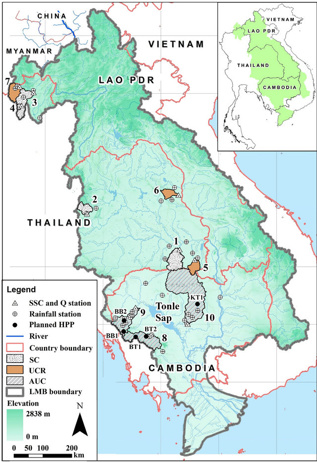
Figure 1. Location map of the study catchments.
employed for model simulation; 2) The UCR containing Catchment No. 5, 6 and 7, was employed for examining the calibrated ANN (Cal-ANN) models. These two sets of catchment are differentiated by the length of data availability: 14 - 20 years for UCR and 20 - 25 years for SC. These seven catchments were selected based on data availability and different geographical/terrain coverage. The Tonle Sap River is a main tributary of the Lower Mekong River and drains about 86,045 km2, 14% of the whole LMB area. The Tonle Sap River Basin (TSRB) is a combined lake and river system of major importance to Cambodia, e.g. water, food and power supply, flood protection, etc. In the TSRB, five HPPs (Figure 1) were planned, two in Catchment No. 8, two in Catchment No. 9 and one in Catchment No. 10 [29]. These three catchments are ungauged in term of sediment data and they are called the AUC in this study. Thus, sediment quantification in these areas is so challenging and important for not only the project development but also the impact assessment on downstream biological system.
2.2. Data
The main data used in this study are suspended sediment load (SSL), discharge (Q), rainfall (R) and digital elevation map (DEM). SSL is the product of Q and SSC. Land use/cover and soil type were accounted for understanding the geo-physical information of each catchment and were not involved in model prediction. The daily data of SSC, Q and R were collected from Mekong River Commission (MRC). As a result from double mass curve plotting, the considered rainfall dataset of each station was confirmed reliable. DEM (30-m resolution) was downloaded from ASTER GDEM 2 [30]. ASTER GDEM is a product of METI and NASA. Land use/cover and soil map were respectively extracted from GLC2000 database [31] and SOIL-FAO database [32].
Daily time series of Q and R are continuous with long term records. SSC time series are discontinuous with low sampling frequency, between 2 and 4 samples per month in average (Table 1), and this provokes the analysis in monthly basis. The monthly average SSL (SSLm) is the product of monthly average Q (Qm) and monthly average SSC (SSCm). The distribution of monthly average R (Rm) over each catchment was conducted using Thiessen Polygon method. Qm and Rm were used as input data for model calculation and SSLm was employed for comparison with the model output. DEM was applied for catchment delineation and slope computation. For model simulation (SC-1, SC-2, SC-3 and SC-4), the whole dataset was divided into two parts: the first 75% for calibration and the remaining 25% for validation. The input combination (75*25%) was decided based on many existing case studies of sediment simulation as summarized in Table 2.
The changes in land use over the simulation period (about 20 years) might cause significant variation of sediment load temporally. This effect could lead to low accuracy of the prediction results. In addition, other human activities could involve in this problem as well. These issues were not considered in the present study due to data constraint. However, the Mann-Kendall test [45, 46] for gradual trend analysis and the Pettitt test [47] for abrupt change detection were applied to examine the time series of annual SSL of each SC. The results of the Mann-Kendall test (Table 3) show that there are no significant trends detected at any of the four SCs at both 0.01 and 0.05 significance level. For the Pettitt test (Table 3), only SSL series of the SC-4 exhibits abrupt change (in 1993) if considering a significance level of 0.05. At significance level of 0.01, there is no change point detected at all SCs. In order to make the model simulation procedures straightforward, significance level of 0.01 was taken into account and therefore, the above mentioned effects were concluded to have no significant influence on the SSL data used for all simulations.
2.3. Artificial Neural Network (ANN)
ANN is characterized by network architecture (pattern of
Table 1. Hydrological and terrain characteristics of the study catchments.

Simulated catchment (SC): 1, 2, 3 and 4; Ungauged catchment representative (UCR): 5, 6 and 7; Actual ungauged catchment (AUC): 8, 9 and 10; aNo data in 1986 and 1987; bNo data in 1995 and 1996; SSLA figures in bold are the model results.
Table 2. Input combination for sediment modeling (Existing case studies).
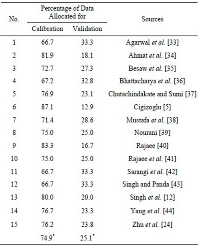
*Average value.
Table 3. Results of the Mann-Kendall and Pettitt test for SSL series of each SC.
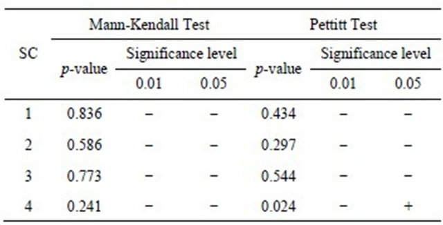
(+) Significant; (−) Not significant.
node-interconnection), method of determining weights on the connections (training algorithm), and transfer function (for generating output). ANN is a broad term covering a large variety of network architectures, the most common of which is a multi-layer perceptron (MLP) [10]. Kisi [7] compared different types of ANN for sediment prediction in Tongue River (Montana, USA) and found that MLP generally yields better results than others. Maier and Dandy [21] reviewed 43 papers dealing with ANN application in water resource modeling and reported that the vast majority considered the backpropagation algorithm for system training. As presented in Figure 2, this study took into account the MLP (1
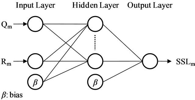
Figure 2. ANN model structure used in this study.
input, 1 hidden and 1 output layer) with the back-propagation algorithm. Due to data limitation, the input layer was designed with two nodes: Qm and Rm. Since there is no fixed rule, the size of hidden layer was determined by trial and error procedure. The single node of the output layer is SSLm. Initially, the input neuron receives a set of inputs (x). The connections between the input and hidden layer contain weights (w) which are determined through the system training. Then, the hidden layer calculates the weighted average of inputs (z) using summation functions:
 (1)
(1)
where wi is the weight vector, xi is the input vector (i = 1, 2, ∙∙∙, n) and β is the bias term. Afterward, the hidden layer uses sigmoid transfer function (Equation (2)) to generate output (y).
 (2)
(2)
Finally, the generated output is compared with the target value. After recognizing the error, the calculation is restarted by adjusting w and this procedure is repeated until obtaining a desirable y. Therefore, ANN model training is the process of weight adjustment that attempts to get a desirable outcome with least squares residuals and the back-propagation is the most common training algorithm.
2.4. Computation Procedure and Model Evaluation
The computation scheme of this study is depicted in Figure 3 and described as below. The designated ANN model was used to simulate SSLm of four SCs. The model architecture (number of hidden nodes) was optimized based on three popularly used statistical indicators: determination coefficient (R2), root mean square error (RMSE) and mean absolute error (MAE). The model efficiency was measured by R2 as well. With R2 greater than 0.50, the model performance is judged satisfactory [48]. In case satisfactory result (R2 > 0.50) is obtained for all SCs, there will be totally four Cal-ANN models which could be applied to estimate SSL in UCs. Since total load (SSLT) is essential for dam-reservoir management [7], the model performance for this purpose was also investigated and absolute percentage bias (APBIAS) was utilized in this case. SSLT is the integral of SSLm series within a particular period. For sediment prediction, the model result is considered acceptable with APBIAS less than 55% [48]. R2, RMSE, MAE and APBIAS were calculated using Equation (3), (4), (5) and (6), respectively.
 (3)
(3)
 (4)
(4)
 (5)
(5)
 (6)
(6)
where X is the observed SSLm with the mean value Xavg, Y is the predicted SSLm with the mean value Yavg, N is the sample size, XT is the observed SSLT, and YT is the predicted SSLT.
Catchment similarity was used to select the most appropriate Cal-ANN for predicting SSLm of UCRs. In this regard, the catchment similarity refers to annual discharge per unit area (QA), annual catchment rainfall (RA) and catchment slope (S). As mentioned earlier, discharge and rainfall are the main erosion and transport agents. Catchment slope or topography is a very important factor controlling land surface erosion and it is included in many erosion prediction methods and mostly the processand physically-based models [8,9]. All three catchment similarity parameters (CSP), QA, RA and S, were used alternately to select a Cal-ANN model for estimating SSLm of three UCRs. In this case, R2 was also employed to evaluate the model efficiency. At the same time, the model performance for SSLT prediction was also investigated using APBIAS. The corresponding R2 (SSLm prediction) of each CSP was afterward compared with each other so as to identify the most ideal CSP. In order to emphasize the consistency, the same procedure was conducted for APBIAS (SSLT prediction).
After identifying the most ideal CSP, it was then used to select an appropriate Cal-ANN for estimating SSLm of three AUCs. The estimated SSLm series was integrated to obtain SSLA. The computed SSLA in this case does not consider the impact of dam-reservoirs. SSLA under the impact of dam-reservoirs (the latter called SSLA*) was calculated by:
 (7)
(7)
where the unit of SSLA in this case is [t/year] and SSLTE is
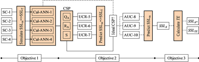
Figure 3. Computation scheme.
the annual SSL trapped by dam-reservoir and it is computed by:
 (8)
(8)
where AR is the drainage area of the dam-reservoir, the unit of SSLA in this case is [t/year/km2] and TE is the reservoir trapping efficiency and it is estimated using Brune’s equation [49]:
 (9)
(9)
where I is the annual discharge at the location of damreservoir and C is the active storage capacity. I and C data were obtained from the Lower Mekong Hydropower Database [29].
The Brune method was originally developed for reservoirs in the United States but it has been widely used as well for other parts of the world such as the Mekong River Basin in Southeast Asian countries plus China and Myanmar [4], the Changjiang River Basin in China [50], the Satluj River Basin in India [51], and so on. For example, the theoretical TE of the Three Gorges Dam on the upper Changjiang River is between 0.73 and 0.78 and this approximates the real TE of 0.75 [50]. The present study considered Brune’s technique because: 1) it is simple and does not require detailed data of the reservoir or sediment which are extremely scarce in the LMB; 2) it is commonly used and found to provide reasonable estimates of long-term, mean TE [9,52]; and 3) it is applied in various studies in the Mekong region and provided acceptable results in comparing with the observed TE values (e.g. Kummu et al. [4], Kummu and Varis [53], Fu and He [54]). For the case study of Manwan Dam in the Upper Mekong Basin, the computed TE value (0.68) using this method is found comparable with the observed one (0.75) [53].
3. Results and Discussion
3.1. Descriptive Statistic of Input Data
Table 4 shows the coefficient of variation (COV), coefficient of skewness (SKEW) and coefficient of kurtosis
Table 4. Statistical characteristics of the data used in this study.

COV: Coefficient of variation; SKEW: Coefficient of skewness; KURT: Coefficient of kurtosis.
(KURT) of the data used in the study. SKEW characterizes the degree of asymmetry of a data distribution while KURT indicates the peakedness or flatness. SSLm datasets are characterized by the largest value of COV (1.44 - 2.47), SKEW (1.93 - 4.91) and KURT (3.10 - 37.00) for all the river systems. This reflects the high temporal variability and non-normal distribution of sediment erosion/transport in nature. That why it is more difficult to be predicted, in comparing with other hydrological variables (e.g. discharge and rainfall). Values of Rm dataset generally showed a near normal distribution with lower values of SKEW and KURT. For model inputs (Qm and Rm), among four SCs, the SC-2 overall contains higher values of COV, SKEW and KURT indicating their high variation and non-normal distribution. This could cause poor calibration performance by the ANN model leading to convergence problems [11].
The distribution of rainfall is primarily driven by topography and the general approach direction of the southwest monsoon. Rainfall in the SC-2 is influenced by the southwest monsoon (May-October) blowing from Bay of Bengal bringing humid and hot weather to the area. Natural topography and mountain ranges make this catchment oriented in a leeward direction creating a rain shadow and therefore, less rainfall amount in comparing with other catchments. The monthly rainfall pattern (1982- 2003) in the SC-2 is characterized by a double peak (one in May and another in September) and this reveals the high variation of rainfall in the area. The double peak of rainfall is due to depressions and typhoons (AugustSeptember) from South China Sea during some years, which brought local heavy rainfall. The high variability in rainfall could be due to local topographic influences as well [27]. This could explain also the great variation and non-normal distribution of the corresponding discharge dataset.
3.2. Model Simulation
In comparing with the observed data, results of the SSLm prediction are graphically shown in Figure 4 (left). It is apparent that trend of the predicted SSLm follows well the observed data in all the years for all four SCs. Figure 4 (right) depicts the scatter plots of the predicted versus observed SSLm which were used to distinguish the ANN performance in low, medium and high value estimation. Overall, the model underestimates the high SSLm values and this might be due to different non-linear relationships governing the sediment erosion and/or transport processes. It is in conformity with findings of various existing researches [11,12,25,55,56] and could be concluded as a common drawback of the ANN model. For low and medium values, the scattered points are distributed uniformly around the ideal fit line.
The model performance for SSLm simulation of each SC is summarized in Table 5. The optimum ANN architecture is 2-5-1, 2-2-1, 2-3-1 and 2-8-1 for SC-1, SC-2, SC-3 and SC-4, respectively. For all SCs, the model performance was judged satisfactory because R2 values are greater than 0.50 in both calibration and validation stage. In calibration period, R2 increases from 0.81 (SC-1) to 0.94 (SC-4); in addition, SC-2 contains much larger error in term of RMSE and MAE, in comparing with other SCs. This could be explained by the statistical characteristics of the input data (Qm and Rm) of each SC. The inputs characterized by higher values of COV, SKEW and KURT are generally more difficult to be calibrated and therefore lower accuracy of the model results. In validation stage, R2 increases from 0.63 (SC-4) to 0.87 (SC-3). There is no common pattern between the model architecture and its performance. However, the model performance indicated by R2 (calibration stage) exhibits good relationship with the catchment topography represented by average slope of the catchment in this study. For SSLT prediction, the model results were also considered acceptable for all cases because APBIAS values are less than 55% in both calibration and validation period. APBIAS is less than 2% in calibration stage and it is less than 40% in validation stage.
From this result, it can be concluded that ANN model performed well in simulating SSLm of various catchments with different hydrological and terrain characteristics. This good result strongly encourages the present authors to apply further the ANN model in UCs in the same region, the LMB. The Cal-ANN models of all SCs were then employed to predict SSLm of three UCRs. There are totally four Cal-ANNs which are Cal-ANN-1 of the SC-1, Cal-ANN-2, Cal-ANN-3 and Cal-ANN-4.
3.3. Assessment of the Cal-ANN Application in UCRs
Among four Cal-ANNs, the most appropriate one was
Table 5. ANN model performance in simulating SSLm of each SC.
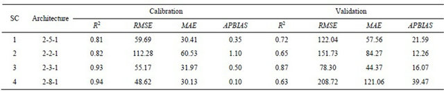
RMSE, MAE: 10-3 t/day/km2; APBIAS: %; R2, RMSE and MAE for SSLm; APBIAS for SSLT; Architecture (optimum): Number of nodes in the Input-HiddenOutput layer.
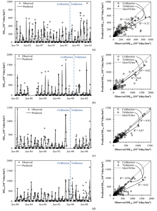
Figure 4. Comparison of the predicted versus observed SSLm of each SC (left) and their scatter plot (right). (a) SC-1; (b) SC-2 (no data in 1986 and 1987); (c) SC-3 (no data in 1995 and 1996); and (d) SC-4.
selected to predict SSLm of three UCRs using three different CSPs (QA, RA and S) alternately. Each CSP was assessed by the model performance in predicting SSLm (R2) and SSLT (APBIAS). For the case using S, CalANN-1 is the most suitable model for the UCR-5, CalANN-2 for the UCR-6 and Cal-ANN-3 for the UCR-7. For example, Cal-ANN-3 of the SC-3 was selected for the UCR-7 because these two catchments have the most similar catchment slope (S). The absolute difference in S value (1.49 = |25.78 − 27.27|) of both catchments is the smallest one in comparing with other cases: 16.35 for (UCR-7 vs SC-1), 3.29 for (UCR-7 vs SC-2) and 6.72 for (UCR-7 vs SC-4). In case of QA and RA, the selected Cal-ANN for each UCR is tabulated in Table 6. From Table 6, it is apparent that the selected Cal-ANNs performed well (R2 > 0.50) in predicting SSLm for all cases. The range of R2 is 0.56 - 0.64, 0.54 - 0.61 and 0.59 - 0.64 for the case using QA, RA and S, correspondingly. Based on the average value of R2 (R2*), catchment slope (S) is the most ideal CSP in identifying the Cal-ANN models. R2* is equal to 0.61 for the case using S and it is about 3% and 5% larger than that of QA and RA case, respectively.
For SSLT prediction, satisfactory results are obtained for only UCR-5 (APBIAS = 1.38%) and UCR-6 (APBIAS = 26.24%) but not UCR-7 (APBIAS = 74.58%) if considering S as the CSP. For the case using QA and RA, the model performance for each UCR is tabulated in Table 6. The range of APBIAS is 8.85% - 97.19%, 22.94% - 204.52% and 1.38% - 74.58% for the case using QA, RA and S, correspondingly. Moreover, the average value of APBIAS (APBIAS*) demonstrates that S is the most ideal CSP in selecting the Cal-ANN models and the second ideal one is QA. For the case using RA, the model yielded unacceptable result with APBIAS* (=95.96%) larger than 55%.
Catchment slope (S) shows its better response repeatedly in selecting the Cal-ANNs of SCs for predicting SSLm and SSLT of UCRs. Physically, sediment production rate of a catchment depends mainly on erodibility of the soil, and erosivity and transport capacity of the discharge. Steep ground surface is generally exposed to high soil erodibility. High erosive force and transport capacity of the discharge is corresponding to high flow velocity which usually occurs in steep slope areas. From this physical aspect, catchment slope or topography governs not only soil erodibility but also pattern of the discharge which drives sediment erosion and transport. In consequence, S is more important than other CSPs.
If the analysis is conducted catchment by catchment, opposition usually occurs. For instance, in the UCR-5, the superior CSP is RA in term of R2 but it turns to S in term of APBIAS. Similarly in the UCR-7, the best CSP is S in term of R2 but it changes to QA in term of APBIAS. According to the overall evaluation indicated by R2* and APBIAS*, S was considered as the most ideal CSP. This conclusion was made based on three UCRs. It is understood that more UCRs should be added in order to make a stronger conclusion. However, data limitation restricts this study to be based on only these three UCRs. By the way, this conclusion could be acceptable because not only one indicator but two (R2 for SSLm and APBIAS for SSLT) were taken into account and both of them provided the same result.
Results of the predicted SSLm series (Cal-ANN was selected based on S) of each UCR are graphically compared with the observed values as shown in Figure 5" target="_self"> Figure 5 (left). It can be seen that both series show similar trend temporally. Based on the scatter plot of the predicted versus observed SSLm (Figure 5 (right)), the model underestimates the high values for the UCR-5 and UCR-6 but overestimates for the UCR-7. This may be due to the fact that Cal-ANN-3 was developed using dataset (COV = 1.67) including extremely low and high SSLm values higher than the one of UCR-7 does (COV = 1.54). In case of Cal-ANN-1 and Cal-ANN-2, their COV value is correspondingly lower than that of UCR-5 and UCR-6, and therefore underestimation of the high values. For low and medium value prediction, the scattered points are distributed around the ideal fit line.
In short, the applicability of ANN model in UCs was proved and catchment slope (S) is the most ideal CSP in selecting the Cal-ANN models for application in UCs. By applying the Cal-ANNs, SSLm and SSLT of UCs
Table 6. Selection of the Cal-ANN model and its performance in predicting SSLm and SSLT of each UCR.
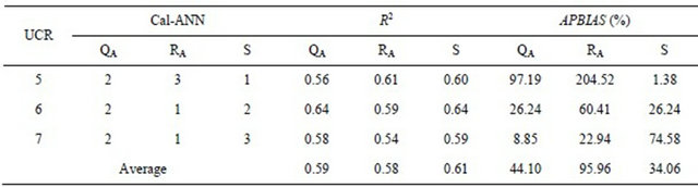
R2 for SSLm; APBIAS for SSLT.
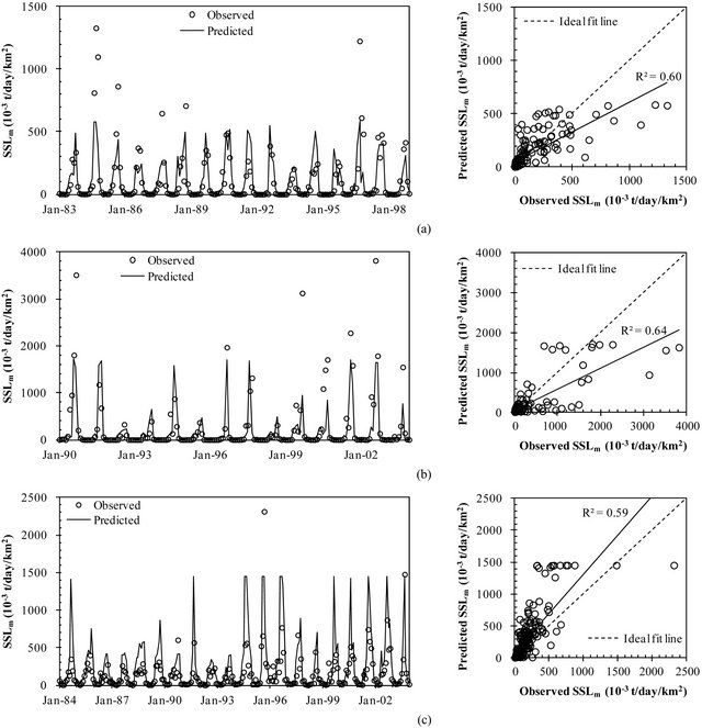
Figure 5. Comparison of the predicted versus observed SSLm of each UCR (left) and their scatter plot (right). (a) UCR-5; (b) UCR-6; and (c) UCR-7.
could be predicted with an accuracy of R2 of 0.61 and APBIAS of 34.06%, respectively.
3.4. Application of the Cal-ANN Models in AUCs
Based on the most ideal CSP (S), Cal-ANN-2 was selected for estimating SSLm of AUC-8 and AUC-9, and Cal-ANN-1 for the AUC-10. The estimated SSLm series was used to compute SSLA. As a result, AUC-8, AUC-9 and AUC-10 produces SSLA around 159,281, 258,943 and 723,580 t/year, respectively. As illustrated in Figure 6, the computed SSLA of AUCs and the observed ones of SCs and UCRs exhibit good relationship with not only the annual discharge but also the catchment area. This reveals the consistent results predicted by the Cal-ANN models. Table 7 presents the SSLA* estimations for each AUC. The estimated SSLA* is 84,608 t/year for the AUC-8, 112,588 t/year for the AUC-9 and 228,610 t/year for the AUC-10. Development of the proposed HPPs could reduce SSLA of AUC-8, AUC-9 and AUC-10 about 47%, 57% and 68%, correspondingly, due to dam-reservoir trapping. This reduction could cause degradation of downstream river channels, decrease of agriculture and fishery production, alteration of catchment biology, and so on. Therefore, this result could be very useful information for water resource managers and different stakeholders for developing the proposed HPPs in a sustainable manner.
Table 7. SSLA* estimation for each AUC.
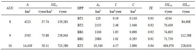
A: Catchment area; AR: Drainage area of dam-reservoir; C: Active storage capacity of dam-reservoir; I: Annual discharge at the location of dam-reservoir; SSLTE: Annual SSL trapped by dam-reservoir; SSLA: Annual SSL (without dam-reservoirs); SSLA*: Annual SSL (with dam-reservoirs); TE: Reservoir trapping efficiency.

Figure 6. Illustration of QA-SSLA and A-SSLA relationship.
4. Conclusions
ANN model performed well in simulating SSLm of four SCs having different hydrological and terrain characteristics. It was calibrated better with input data having less variation and near normal distribution. Moreover, its performance (R2) was superior with catchments characterized by steeper slope. The Cal-ANN models were applied to predict SSLm of three UCRs and at the same time, their performance in predicting SSLT was also investigated. Three different CSPs were used alternately to select the most appropriate Cal-ANN for each UCR. The analysis showed that catchment slope (S) is the most ideal CSP. Based on these two observations on S, it can be concluded that parameters of the Cal-ANN models might contain some physical information governing the catchment topography. The Cal-ANN model performance in UCRs was considered acceptable for both SSLm and SSLT prediction. Using these models, SSLm and SSLT of UCs in this region (LMB) could be predictable at an accuracy of 0.61 in term of R2 and 34.06% in term of APBIAS, respectively. In combination with Brune’s method, one can estimate sediment load which could be trapped by the planned dam-reservoirs and remain flowing to downstream. This information is very important for sustainability of such developments. The model application in the TSRB could be a good example in this regard.
In this study, only four Cal-ANN models were established. Consequently, with other UCs characterized by S different significantly from the considered four SCs, the prediction results might contain high uncertainty. Therefore, more Cal-ANNs should be built up. However, this finding is a key step providing high motivation for further study.
5. Acknowledgements
Sincerest thank is deeply expressed to Japanese Government (Monbukagakusyo: MEXT) and Global Center of Excellent program of University of Yamanashi, Japan, for supporting this research study.
REFERENCES
- D. E. Walling and D. Fang, “Recent Trends in the Suspended Sediment Loads of the World’s Rivers,” Global and Planetary Change, Vol. 39, No. 1-2, 2003, pp. 111- 126. doi:10.1016/S0921-8181(03)00020-1
- Z. Babinski, “The Relationship between Suspended and Bed Load Transport in River Channels,” International Symposium on Sediment Budgets, Foz do Iguaço, 3-9 April 2005, pp. 182-188.
- MRC (Mekong River Commission), “Transboundary River Basin Management: Addressing Water, Energy and Food Security,” MRC, Vientiane, 2012.
- M. Kummu, X. X. Lu, J. J. Wang and O. Varis, “BasinWide Sediment Trapping Efficiency of Emerging Reservoirs along the Mekong,” Geomorphology, Vol. 119, No. 3-4, 2010, pp. 181-197. doi:10.1016/j.geomorph.2010.03.018
- H. K. Cigizoglu, “Estimation and Forecasting of Daily Suspended Sediment Data by Multi-Layer Perceptrons,” Advances in Water Resources, Vol. 27, No. 2, 2003, pp. 185-195. doi:10.1016/j.advwatres.2003.10.003
- A. J. Horowitz, “An Evaluation of Sediment Rating Curves for Estimating Suspended Sediment Concentrations for Subsequent Flux Calculations,” Hydrological Processes, Vol. 17, No. 17, 2003, pp. 3387-3409. doi:10.1002/hyp.1299
- O. Kisi, “Multi-Layer Perceptrons with Levenberg-Marquardt Training Algorithm for Suspended Sediment Concentration Prediction and Estimation,” Hydrological Sciences Journal, Vol. 49, No. 6, 2004, pp. 1025-1040. doi:10.1623/hysj.49.6.1025.55720
- USBR (United States Bureau of Reclamation), “Erosion and Sedimentation Manual,” USBR, Colorado, 2006.
- G. L. Morris and J. Fan, “Reservoir Sedimentation Handbook: Design and Management of Dams, Reservoirs, and Watershed for Sustainable Use,” McGraw-Hill, New York, 1998.
- O. M. Rezapour, L. T. Shui and D. B. Ahmad, “Review of Artificial Neural Network Model for Suspended Sediment Estimation,” Australian Journal of Basic and Applied Sciences, Vol. 4, No. 8, 2010, pp. 3347-3353.
- A. M. Melesse, S. Ahmad, M. E. McClain, X. Wang and Y. H. Lim, “Suspended Sediment Load Prediction of River Systems: An Artificial Neural Network Approach,” Agricultural Water Management, Vol. 98, No. 5, 2011, pp. 855-866. doi:10.1016/j.agwat.2010.12.012
- A. Singh, M. Imtiyaz, R. K. Isaac and D. M. Denis, “Comparison of Soil and Water Assessment Tool (SWAT) and Multilayer Perceptron (MLP) Artificial Neural Network for Predicting Sediment Yield in the Nagwa Agricultural Watershed in Jharkhand, India,” Agricultural Water Management, Vol. 104, 2011, pp. 113-120. doi:10.1016/j.agwat.2011.12.005
- O. Kisi and J. Shiri, “River Suspended Sediment Estimation by Climatic Variables Implication: Comparative Study among Soft Computing Techniques,” Computers & Geosciences, Vol. 43, 2012, pp. 73-82. doi:10.1016/j.cageo.2012.02.007
- J. J. Wang, X. X. Lu and M. Kummu, “Sediment Load Estimates and Variations in the Lower Mekong River,” River Research and Applications, Vol. 27, No. 1, 2009, pp. 33-46. doi:10.1002/rra.1337
- C. T. Yang, “Incipient Motion and Sediment Transport,” Journal of the Hydraulics Division, Vol. 99, No. 10, 1973, pp. 1679-1704.
- J. M. Wicks and J. C. Bathurst, “SHESED: A Physically Based, Distributed Erosion and Sediment Yield Component for the SHE Hydrological Model System,” Journal of Hydrology, Vol. 175, No. 1-4, 1996, pp. 213-238. doi:10.1016/S0022-1694(96)80012-6
- N. E. M. Asselman, “Fitting and Interpretation of Sediment Rating Curves,” Journal of Hydrology, Vol. 234, No. 3-4, 2000, pp. 228-248. doi:10.1016/S0022-1694(00)00253-5
- J. A. Warrick and D. M. Rubin, “Suspended-Sediment Rating Curve Response to Urbanization and Wildfire, Santa Ana River, California,” Journal of Geophysical Research, Vol. 112, No. F2, 2007, Article ID: F02018. doi:10.1029/2006JF000662
- J. R. Williams, “Sediment Yield Prediction with Universal Equation Using Runoff Energy Factor, in Present and Prospective Technology for Predicting Sediment Yields and Sources, ARS-S-40,” USDA, Washington DC, 1975.
- S. L. Neitsch, J. G. Arnold, J. R. Kiniry and J. R. Williams, “Soil and Water Assessment Tool,” Texas Water Resources Institute, Texas, 2011.
- H. R. Maier and G. C. Dandy, “Neural Networks for the Prediction and Forecasting of Water Resources Variables: A Review of Modelling Issues and Applications,” Environmental Modelling & Software, Vol. 15, No. 1, 1999, pp. 101-124. doi:10.1016/S1364-8152(99)00007-9
- V. Nourani, O. Kalantari and A. Baghanam, “Two Semidistributed ANN-Based Models for Estimation of Suspended Sediment Load,” Journal of Hydrologic Engineering, Vol. 17, No. 12, 2012, pp 1368-1380. doi:10.1061/(ASCE)HE.1943-5584.0000587
- G. Tayfur, “Artificial Neural Networks for Sheet Sediment Transport,” Hydrological Sciences Journal, Vol. 47, No. 6, 2002, pp. 879-892. doi:10.1080/02626660209492997
- Y. M. Zhu, X. X. Lu and Y. Zhou, “Suspended Sediment Flux Modeling with Artificial Neural Network: An Example of the Longchuangjiang River in the Upper Yangtze Catchment, China,” Geomorphology, Vol. 84, No. 1-2, 2006, pp. 111-125. doi:10.1016/j.geomorph.2006.07.010
- M. Talebizadeh, S. Morid, S. A. Ayyoubzadeh and M. Ghasemzadeh, “Uncertainty Analysis in Sediment Load Modeling using ANN and SWAT Model,” Water Resources Management, Vol. 24, No. 9, 2009, pp. 1747- 1761. doi:10.1007/s11269-009-9522-2
- H. K. Cigizoglu, “Suspended Sediment Estimation for Rivers Using Artificial Neural Networks and Sediment Rating Curves,” Turkish Journal of Engineering and Environmental Sciences, Vol. 26, No. 1, 2002, pp. 27-36.
- MRC (Mekong River Commission), “Planning Atlas of the Lower Mekong River Basin,” MRC, Phnom Penh and Vientiane, 2011.
- H. J. Fuchs, “Data Availability for Studies on Effects of Land-Cover Changes on Water Yield, Sediment and Nutrient Load at Catchments of the Lower Mekong Basin,” MRC-GTZ Cooperation Programme, Göttingen, 2004.
- MRC (Mekong River Commission), “Lower Mekong Hydro Power Database,” MRC, Vientiane, 2009.
- METI and NASA (Ministry of Economy, Trade and Industry, Japan, and National Aeronautics and Space Administration), “Advanced Spaceborne Thermal Emission and Reflection Radiometer: Global Digital Elevation Model Version 2,” 2011. http://www.jspacesystems.or.jp/ersdac/GDEM/E/4.html
- EC-JRC (European Commission Joint Research Center), “The Land Cover Map for South East Asia in the Year 2000,” 2003. http://bioval.jrc.ec.europa.eu/products/glc2000/products.php
- FAO (Food and Agriculture Organization of the United Nations), “The Digital Soil Map of the World,” 2003. http://www.fao.org/geonetwork/srv/en/metadata.show?id=14116
- A. Agarwal, R. K. Rai and A. Upadhyay, “Forecasting of Runoff and Sediment Yield Using Artificial Neural Networks,” Journal of Water Resource and Protection, Vol. 1, No. 5, 2009, pp. 368-375. doi:10.4236/jwarp.2009.15044
- N. N. I. Ahmat, S. Harun, J. Ariffin and S. Abdul-Talib, “Sediment Transport Prediction by Using 3-Layer Feedforward MLP Networks,” The 11th International Conference on Urban Drainage, Edinburgh, 31 August-5 September 2008.
- L. E. Besaw, D. M. Rizzo, P. R. Bierman and W. R. Hackett, “Advances in Ungauged Streamflow Prediction Using Artificial Neural Networks,” Journal of Hydrology, Vol. 386, No. 1-4, 2010, pp. 23-37. doi:10.1016/j.jhydrol.2010.02.037
- B. Bhattacharya, R. K. Price and D. P. Solomatine, “DataDriven Modelling in the Context of Sediment Transport,” Physics and Chemistry of the Earth, Vol. 30, No. 4-5, 2005, pp. 297-302. doi:10.1016/j.pce.2004.12.001
- C. Chutachindakate and T. Sumi, “Sediment Yield and Transportation Analysis: Case Study on Managawa River Basin,” Annual Journal of Hydraulic Engineering, Vol. 52, 2008, pp. 157-162. doi:10.2208/prohe.52.157
- M. R. Mustafa, M. H. Isa and R. B. Rezaur, “A Comparison of Artificial Neural Networks for Prediction of Suspended Sediment Discharge in River: A Case Study in Malaysia,” World Academy of Science, Engineering and Technology, Vol. 81, 2011, pp. 372-376.
- V. Nourani, “Using Artificial Neural Networks (ANNs) for Sediment Load Forecasting of Talkherood River Mouth,” Journal of Urban and Environmental Engineering, Vol. 3, No. 1, 2009, pp. 1-6. doi:10.4090/juee.2009.v3n1.001006
- T. Rajaee, “Wavelet and ANN Combination Model for Prediction of Daily Suspended Sediment Load in Rivers,” Science of the Total Environment, Vol. 409, No. 15, 2010, pp. 2917-2928. doi:10.1016/j.scitotenv.2010.11.028
- T. Rajaee, S. A. Mirbagheri, M. Zounemat-Kermani and V. Nourani, “Daily Suspended Sediment Concentration Simulation Using ANN and Neuro-Fuzzy Models,” Science of the Total Environment, Vol. 407, No. 17, 2009, pp. 4916-4927. doi:10.1016/j.scitotenv.2009.05.016
- A. Sarangi, C. A. Madramootoo, P. Enright, S. O. Prasher and R. M. Patel, “Performance Evaluation of ANN and Geomorphology-Based Models for Runoff and Sediment Yield Prediction for a Canadian Watershed,” Current Science, Vol. 89, No. 12, 2005, pp. 2022-2033.
- G. Singh and R. K. Panda, “Daily Sediment Yield Modeling with Artificial Neural Network Using 10-Fold Cross Validation Method: A Small Agricultural Watershed, Kapgari, India,” International Journal of Earth Sciences and Engineering, Vol. 4, No. 6, 2011, pp. 443-450.
- C. T. Yang, R. Marsooli and M. T. Aalami, “Evaluation of Total Load Sediment Transport Formulas Using ANN,” International Journal of Sediment Research, Vol. 24, No. 3, 2009, pp. 274-286. doi:10.1016/S1001-6279(10)60003-0
- H. B. Mann, “Nonparametric Tests against Trend,” Econometrica, Vol. 13, No. 3, 1945, pp. 245-259. doi:10.2307/1907187
- M. G. Kendall, “Rank Correlation Methods,” Griffin, London, 1975.
- A. N. Pettitt, “A Non-Parametric Approach to the ChangePoint Problem,” Applied Statistics, Vol. 28, No. 2, 1979, pp. 126-135. doi:10.2307/2346729
- D. N. Moriasi, J. G. Arnold, M. W. V. Liew, R. L. Bingner, R. D. Harmel and T. L. Veith, “Model Evaluation Guidelines for Systematic Quantification of Accuracy in Watershed Simulations,” Transactions of the American Society of Agriculture and Biological Engineers, Vol. 50, No. 3, 2007, pp. 885-900.
- G. M. Brune, “Trap Efficiency of Reservoirs,” Transactions of the American Geophysical Union, Vol. 34, No. 3, 1953, pp. 407-418. doi:10.1029/TR034i003p00407
- B. Hu, Z. Yang, H. Wang, X. Sun, N. Bi and G. Li, “Sedimentation in the Three Gorges Dam and the Future Trend of Changjiang (Yangtze River) Sediment Flux to the Sea,” Hydrology and Earth System Sciences, Vol. 13, No. 11, 2009, pp. 2253-2264. doi:10.5194/hess-13-2253-2009
- V. Jothiprakash and V. Garg, “Re-Look to Conventional Techniques for Trapping Efficiency Estimation of a Reservoir,” International Journal of Sediment Research, Vol. 23, No. 1, 2008, pp. 76-84. doi:10.1016/S1001-6279(08)60007-4
- C. J. Vorosmarty, M. Meybeck, B. Fekete, K. Sharma, P. Green and J. P. M. Syvitski, “Anthropogenic Sediment Retention: Major Global Impact from Registered River Impoundments,” Global and Planetary Change, Vol. 39, No. 1-2, 2003, pp. 169-190. doi:10.1016/S0921-8181(03)00023-7
- M. Kummu and O. Varis, “Sediment-Related Impacts due to Upstream Reservoir Trapping, the Lower Mekong River,” Geomorphology, Vol. 85, No. 3-4, 2006, pp. 275- 293. doi:10.1016/j.geomorph.2006.03.024
- K. D. Fu and D. M. He, “Analysis and Prediction of Sediment Trapping Efficiencies of the Reservoirs in the Mainstream of the Lancang River,” Chinese Science Bulletin, Vol. 52, No. 2, 2007, pp. 134-140. doi:10.1007/s11434-007-7026-0
- H. Memarian and S. K. Balasundram, “Comparison between Multi-Layer Perceptron and Radial Basis Function Networks for Sediment Load Estimation in a Tropical Watershed,” Journal of Water Resource and Protection, Vol. 4, No. 10, 2012, pp. 870-876. doi:10.4236/jwarp.2012.410102
- T. Rajaee, S. A. Mirbagheri, V. Nourani and A. Alikhani, “Prediction of Daily Suspended Sediment Load Using Wavelet and Neuro-Fuzzy Combined Model,” International Journal of Environmental Science and Technology, Vol. 7, No. 1, 2009, pp. 93-110.