Journal of Water Resource and Protection
Vol.4 No.7(2012), Article ID:19792,8 pages DOI:10.4236/jwarp.2012.47048
Modeling the Effect of Irrigation Practices in Flash Floods: A Case Study for the US Southwest
1Department of Civil Engineering and Engineering Mechanics, The University of Arizona, Tucson, USA
2Department of Hydrology and Water Resources, The University of Arizona, Tucson, USA
Email: camicase7@gmail.com
Received April 20, 2012; revised May 16, 2012; accepted June 2, 2012
Keywords: Irrigation Practices; Flash Flood Events; Reference Crop Evapotranspiration; Soil Saturation; Streamflow Forecasts
ABSTRACT
Conventional streamflow forecasting does not generally take into account the effects of irrigation practice on the magnitude of floods and flash floods. In this paper, we report the results of a study in which we modeled the impacts of an irrigated area in the US Southwest on streamflow. A calibrated version of the Variable Infiltration Capacity model (VIC), coupled with a routing algorithm, was used to investigate two strategies for irrigating alfalfa in the Beaver Creek watershed (Arizona, USA), for the period January to March of 2010, at a resolution of 1.8 km and hourly time step. By incorporating the effects of irrigation in artificially maintaining soil moisture, model performance is improved without requiring changes in the resolution or quality of input data. Peak flows in the watershed were found to increase by 10 to 500 times, depending on the irrigation scenario, as a function of the strategy and the intensity of rainfall. The study suggests that both flood control and irrigation efficiency could be enhanced by applying improved irrigation techniques.
1. Introduction
Floods are the main cause of fatalities from natural hazards in the United States [1]. Further, flash floods are particularly difficult to predict in a timely manner, both in their time of occurrence and magnitude. They are caused by intense rainfall occurring during a relatively short period of time (generally less than 6 hours) and they move quickly through riverbeds, urban areas, or mountain canyons causing considerable devastation along the way [2]. While their occurrence may be caused by the interaction of hydrometeorological and geomorphological factors, their magnitudes can be significantly affected by land use policies and irrigation practices in the drainage area.
The success of any flood warning system (in terms of prevention of casualties and reduced damage) depends on two major analytical components—weather forecasts and rainfall-runoff models informed by proper characterization of the basin. However, conventional streamflow forecasts commonly disregard irrigation contributions to soil moisture. Several authors have studied the impacts of irrigated areas on atmospheric and land-surface variables. Ref [3] modified the Variable Infiltration Capacity (VIC model, [4]) to allow for irrigation to be initiated once soil moisture drops below the level that limits transpiration, and to continue until soil moisture reaches field capacity;
their study focused on the sources of water for irrigation in large basins. Ref [5] simulated the impact of irrigation by forcing the root zone to field capacity at every time step; they observed that land-use change provides a regional climate forcing of opposite sign to that of greenhouse forcing. A similar result was reported by [6], who found that simulating irrigated areas can result in local cooling of up to 8˚C. However most such modeling studies have not included information about the volumes of water added to agricultural areas through irrigation [7].
In the US, forecasting of flash flood events is performed by the National Weather Service (NWS) through its River Forecast Centers (RFC). For the Southwestern US, the NWS Weather Forecast Office (WFO) generates 6-hour precipitation forecasts on an hourly-time step during the monsoon season, based on which RFC forecasters use a catchment model to estimate the streamflow hydrograph. Then, taking into account local topography, land cover, previous rainfall events and flash floods in the area, they decide whether it is necessary to issue a flash flood warning. Because of the potential effects of irrigation practice on streamflow, the NWS has become involved in incorporating, into this analysis, cost-effective techniques for the evaluation of irrigation impacts.
This paper reports on a pilot study designed to investigate the potential impacts of irrigation on streamflow.
The VIC model, with relatively fine spatial resolution was coupled to a routing model and set up to be run at hourly time steps, to generate seven-day forecasts for a catchment in the Southwestern US. We modified the VIC model to incorporate irrigation, and evaluated the effects of two irrigation strategies on the catchment response to precipitation events. Care was taken to represent irrigated areas as accurately as possible. Our approach included the simulation of irrigation practices, information about the amount of water used in irrigation and calibration of the streamflow hydrograph.
2. Methodology
2.1. Study Area
The Beaver Creek sub-basin (Figure 1), encompassing 2000 acres of alfalfa [8], was chosen for this study because it isolates the real effect of irrigation in the US Southwest by being the only irrigated land within the Verde River basin. Beaver Creek characterizes a typical US Southwest hydrological system, linking together perennial and ephemeral regimes, drought, flood and fire cycles, and surface flow and groundwater. There is also snow melting from the winter rains during the spring. The observed hydrograph was obtained from Wet Beaver creek station (USGS 09505200), with a drainage area of 111 square miles (287.5 km2), from January 1st through June 30th, 2010 in hourly time steps. Beaver Creek is represented in the VIC model by 91 grid cells, each of size 1.8 km by 1.8 km.
2.2. The Hydrologic Model
The VIC model, as implemented for this study, uses sub-daily meteorological drivers to compute land-atmosphere fluxes, the water balance (assuming soil surface temperature equals air temperature), and the energy balance (by finding a surface temperature which adjusts surface energy fluxes). The land surface is modeled as a grid of flat, uniform cells and the water/energy balance calculations are done on each grid cell separately. The data for Beaver Creek is available at different spatial and temporal resolutions. Since the VIC model requires all inputs to be provided at the same resolution as the grid cells, all the information was downscaled to 1.8 km and hourly time steps based on topographical attributes and daily and monthly temperature spreads. A soil parameter file defines the soil properties, geographic information, and initial soil moisture conditions for each grid cell, and a vegetation parameter file defines the different land cover types allowed in the simulation, along with the number of vegetation tiles in each grid cell, their areal coverage and land cover type [4]. The only “water” input to the VIC soil column is precipitation (plus, if relevant, snowmelt). The vertical soil column is divided into an arbitrary number of layers: for this study we used two soil layers (a 5 cm thick top layer and a 95 cm thick bottom layer) to represent the whole root zone in a unique layer. Infiltration into the top-most layer is controlled by a “variable infiltration capacity” (VIC) parameterization. The top-most layers can lose moisture through evapotranspiration. Flow is driven by gravity to lower layers. VIC incorporates the ARNO parameterization [9] to represent baseflow drainage from the bottom layer. Streamflow routing is performed separately from the land surface simulation, using a model proposed by [10].
Meteorological drivers and land surface characteristics from Beaver Creek watershed are provided to the coupled VIC-routing model to initiate the simulation (Table 1). The period from January through March of 2010 was used to calibrate the parameters of the model using both Mean Squared Error (MSE) and visual inspection. This calibration will be further used by another research team at The University of Arizona to create more accurate ensemble streamflow forecasts based on a variety of precipitation scenarios [11].

Figure 1. Beaver creek watershed (right) is a tributary of the Verde River basin (middle). The irrigated area of alfalfa is circumscribed within the line in red in beaver creek watershed.
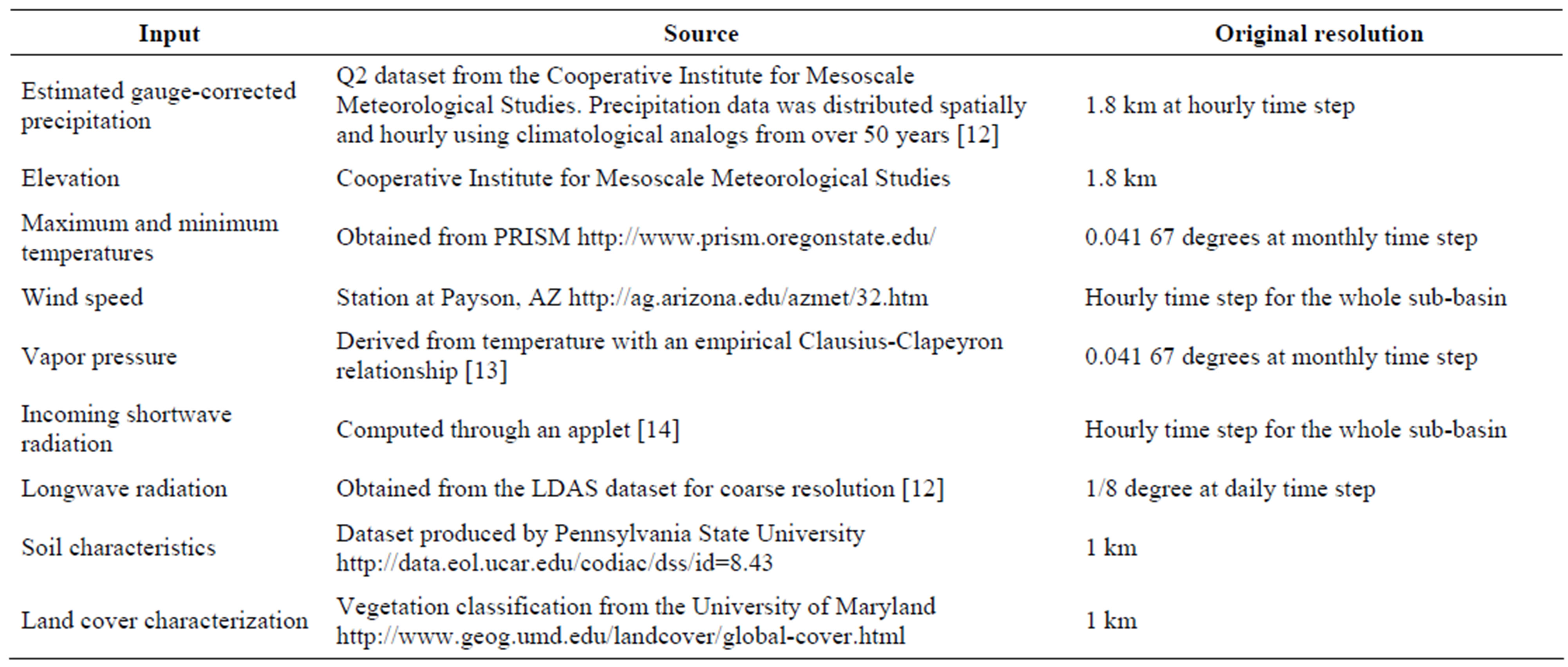
Table 1. Input drivers for beaver creek watershed.
2.3. Calibration Results
As can be seen in Figure 2, the VIC model simulated, acceptably well, the magnitude and time of occurrence of most of the peaks, as well as the seasonal streamflow behavior corresponding to snow melting during March, even when no irrigation is assumed to be occurring. However, while it is able to reproduce the time of occurrence of the flow peak on January 22nd (the main event), its simulation of the event magnitude is significantly lower than that recorded for the event (see the nonirrigated scenario in Figure 2 ).
2.4. Evaluating Effects of Irrigation
2.4.1. Irrigation Strategies Investigated
The effects of two irrigation strategies were considered in this study: 1) Maintaining constant soil moisture, and 2) Constant rate of irrigation. In both cases, irrigation was applied uniformly over the entire grid cell. The areas irrigated correspond to alfalfa fields near Rimrock, AZ (Figure 1). We assume that an unlimited supply of ground-water is available for irrigation.
2.4.2. Inclusion of Alfalfa in the VIC Model
In order to simulate the effects of transpiration from vegetation, the following information for alfalfa was included in the VIC Vegetation library: for areas comprising farmland, the LAI value was set to 2.4, corresponding to light frequent irrigated full-grown alfalfa [15]; albedo values for alfalfa (obtained via remote sensing) lie between 0.25 and 0.62 for clear sky conditions, and vary accordingly to solar altitude angle [16]; roughness (typically 0.123 times vegetation height) and displacement (typically 0.67 times vegetation height) depend on the height of fully grown alfalfa [4], which is normally three feet [17].
2.4.3. Strategy of Maintaining Constant Soil Moisture
A constant field capacity value prevents a plant from wilting, and allows it to optimally utilize soil moisture for growth without deriving excess water to transpiration or baseflow fluxes. In this strategy, water is added to the bottom soil layer at every time step that it drops below a user-specified soil moisture level, so as to resemble those constant field capacity values. Additions of water are considered to occur instantaneously, and the model code was modified to keep track of (and record) the volume of water added at every time step. Eight different soil-moisture saturation levels were investigated, ranging from 10% to 90% saturation. Water was not added to the upper soil layer, because the “variable infiltration capacity” parameterization used in VIC is such that doing so would have the unrealistic effect of causing some of the applied water to run-off into the river.
2.4.4. Strategy of Constant Irrigation Rate
In this strategy, a user-specified constant rate of water was added to the bottom soil layer at every time step. The application amount was computed from each of the eight saturation cases of the previous strategy, to correspond to the average rates of water applied over the period of study. This strategy is more representative of actual irrigation practices, where constant rates are typically applied for several time steps. As a consequence, in this strategy, soil moisture level can temporarily vary both above and below the desired saturation level. Consequently, we define the “effectiveness” of this strategy as being the percentage of time that soil moisture is above or at the saturation level specified. According to this definition, the strategy of maintaining constant soil
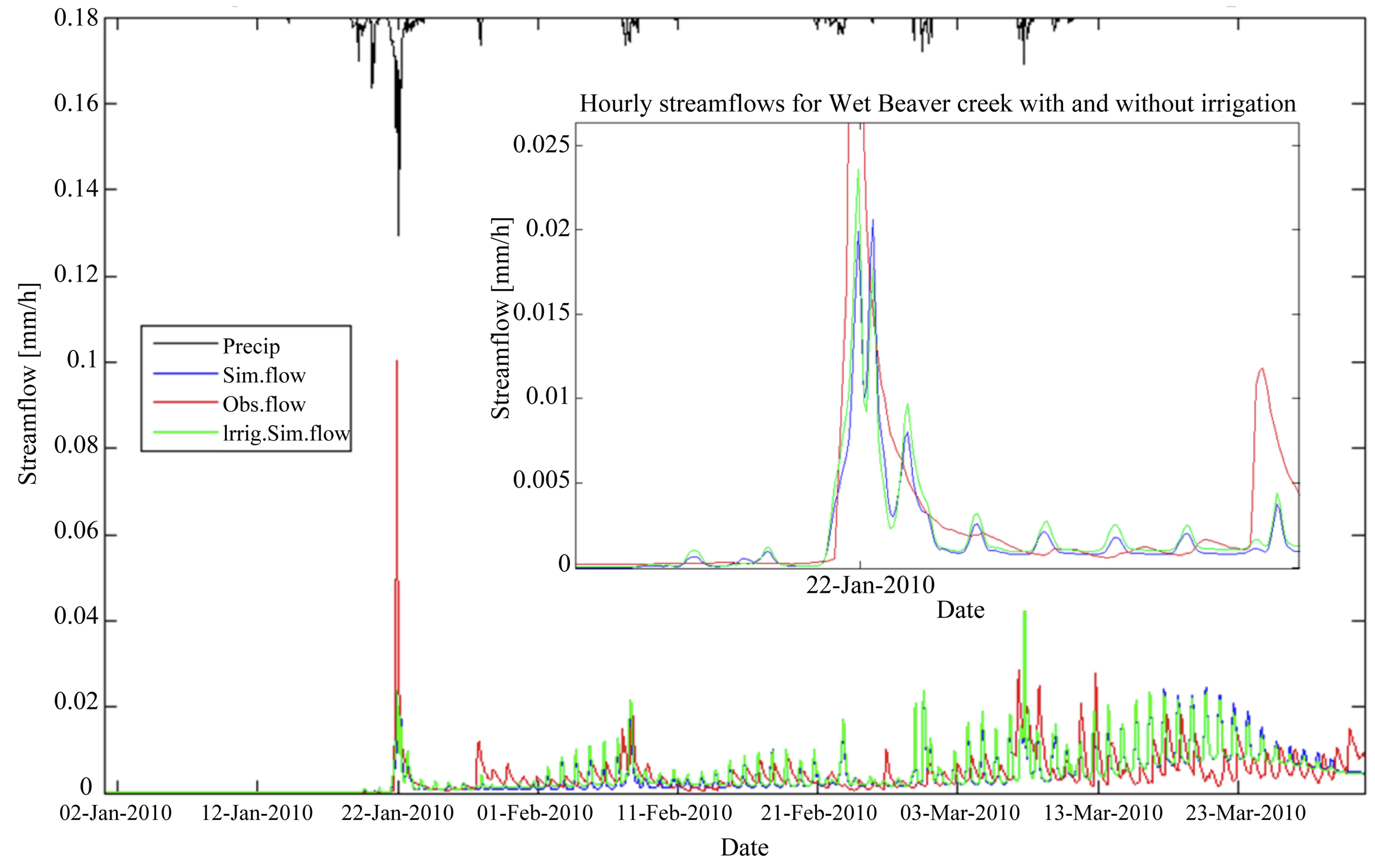
Figure 2. Simulated hydrograph for optimum conditions (green), for non-irrigated scenario (blue), and observed hydrograph (red) in Beaver Creek. The average precipitation in the sub-basin is presented on top (in black). The detail in the box corresponds to the flow peak for the main precipitation event on January 22nd.
moisture has an effectiveness of 100%, whereas effectiveness of the constant rate of irrigation strategy can fall below 100%, particularly for higher desired soil moisture levels, as it is shown in Figure 3.
3. Results
3.1. Impacts of Irrigation on Runoff, Evaporation, and Baseflow
Both the constant soil moisture and constant rate of irrigation strategies show similar trends regarding total cumulative runoff volume, evapotranspiration, and baseflow for the irrigated area under study. Figure 4 shows how these values vary with the different soil moisture saturation level scenarios, for the strategy of constant soil moisture. Cumulative evapotranspiration increases with each scenario until it reaches the reference crop level (50% saturation), representing the maximum soil moisture level that a plant is able to convert into evapotranspiration. For the original non-irrigated scenario and for scenarios up to 30% soil moisture level, precipitation is the main contributor to evapotranspiration, whereas for the higher soil moisture scenarios evapotranspiration is controlled by both precipitation and irrigation. Significant increases in cumulative runoff and baseflow occur for irrigation scenarios where soil moisture is maintained at levels higher than the reference crop level.

Figure 3. Effectiveness of the constant irrigation rate strategy along different user-specified rates of water.
3.2. Impacts of Irrigation on Flow Peaks
Both strategies were found to have similar impacts on the simulated flow peaks throughout the entire period under study (January-March). Exceedance probability was computed for the fifty highest streamflow values in each scenario using the Weibull distribution [18]. Figure 5 shows that significant changes in the magnitude of the largest streamflow values occur for scenarios with soil moisture levels artificially maintained above the reference crop level.
Figure 6 shows the times at which a streamflow value was larger than during the non-irrigation scenario, for different scenarios of the constant soil moisture strategy.
 (a)
(a) (b)
(b)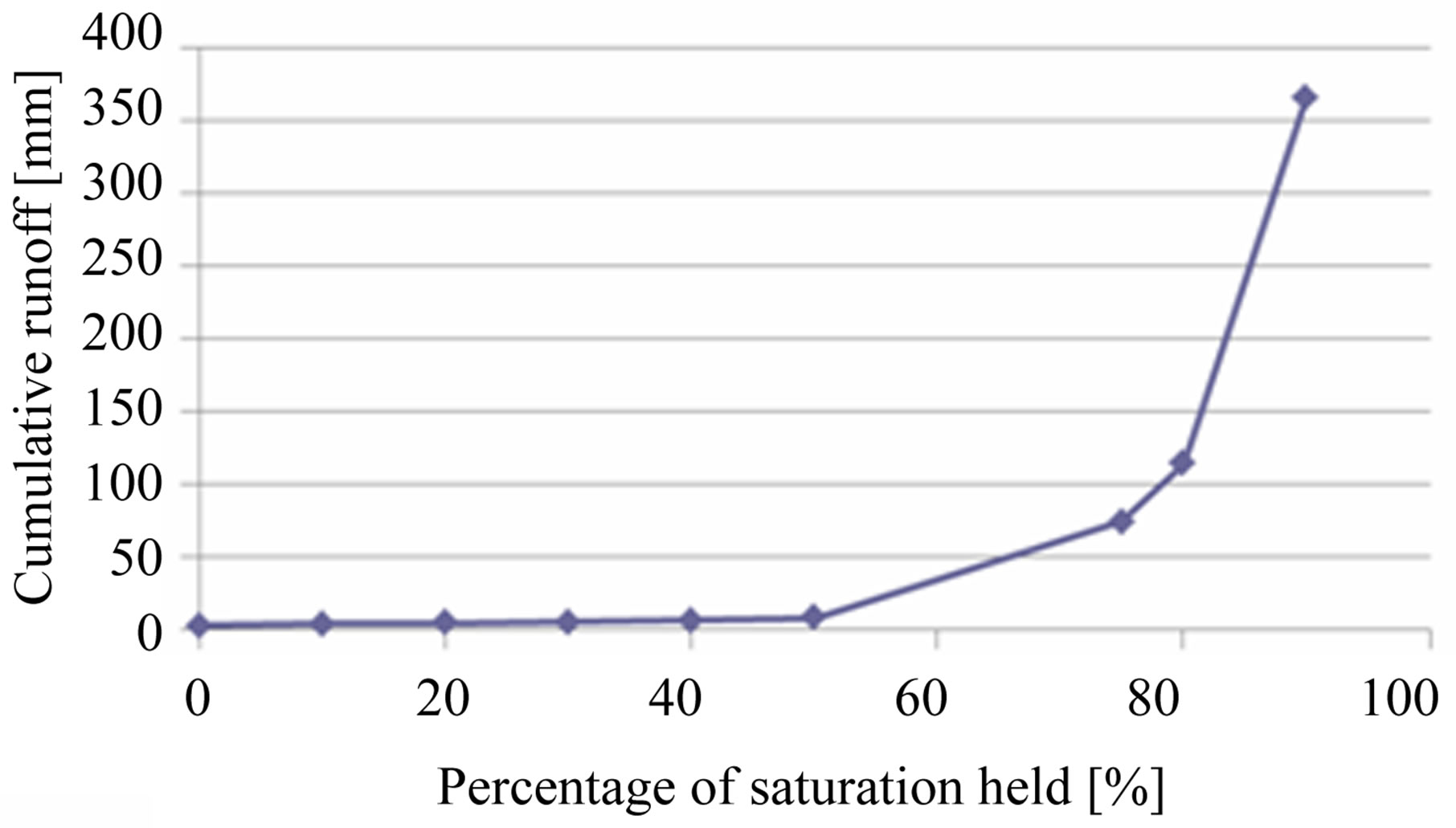 (c)
(c)
Figure 4. Total volume of water in (a) Runoff; (b) Evapotranspiration; and (c) Baseflow, for the different scenarios from Maintained soil moisture strategy.

Figure 5. Probability of exceedance for the 50 largest streamflow values in each scenario from maintained soil moisture strategy. Each line represents a different scenario.
0.0004 0.0008 0.0016 0.0032 0.0064 0.0128 0.0256 Probability of exceedance
In general, the magnitudes of the increases are proportional to the magnitude obtained without irrigation. Notice, however, that the increases in the peak flows for the large storm event in January are several times larger than the other values in the series.
3.3. Simulations for the Whole Basin including Irrigation Scheme
3.3.1. Simulation for Optimum Conditions
The previous results were computed only for a single grid cell, to investigate the kinds of changes we can expect. The registered irrigation area in Beaver Creek (2000 acres) corresponds to at least two grid cells to achieve an equivalent irrigated area (1600 acres). Simulation for optimum conditions of irrigation implies a scenario with soil moisture level at a minimum of 50% saturation (reference crop level) within the strategy of maintaining soil moisture. Simulated hydrographs for these optimum conditions and for the non-irrigated scenario are shown in Figure 2, along with the observed hydrograph and precipitation. This simulation had no observable impact on the values of the hydrograph for the whole sub-basin. However, the inclusion of irrigation increased the cumulative streamflow volume in the subbasin by 0.16 million cubic meters for the whole period (January through March), corresponding to a 6.5% increase over the original simulation volume (no irrigation).
3.3.2. Simulation for Extreme Case
An extreme case for irrigation can be constructed by considering a hypothetical (larger than registered) area represented by four grid cells (3200 acres), over which a constant soil moisture of 90% saturation is maintained. This is clearly a case of “over-irrigation”, since soil moisture is kept well above the reference crop level.
Figure 7 shows that this scenario results in an improved simulation of the observed hydrograph, and especially for the large peak associated with the main precipitation event on January 22nd. The simulated large peak, however, has an attenuation that splits it in two, probably because the model allows a faster infiltration by not taking into account the temporary impermeability of water itself as it runs over the surface. An increase in baseflow is also observed along the three-month period. The total streamflow volume for the basin during the simulation increased in 1.58 million cubic meters, constituting 65% of the original simulation volume (no irrigation).
4. Concluding Remarks
Irrigation practices significantly affect the magnitude of flow peaks produced by precipitation events, especially if
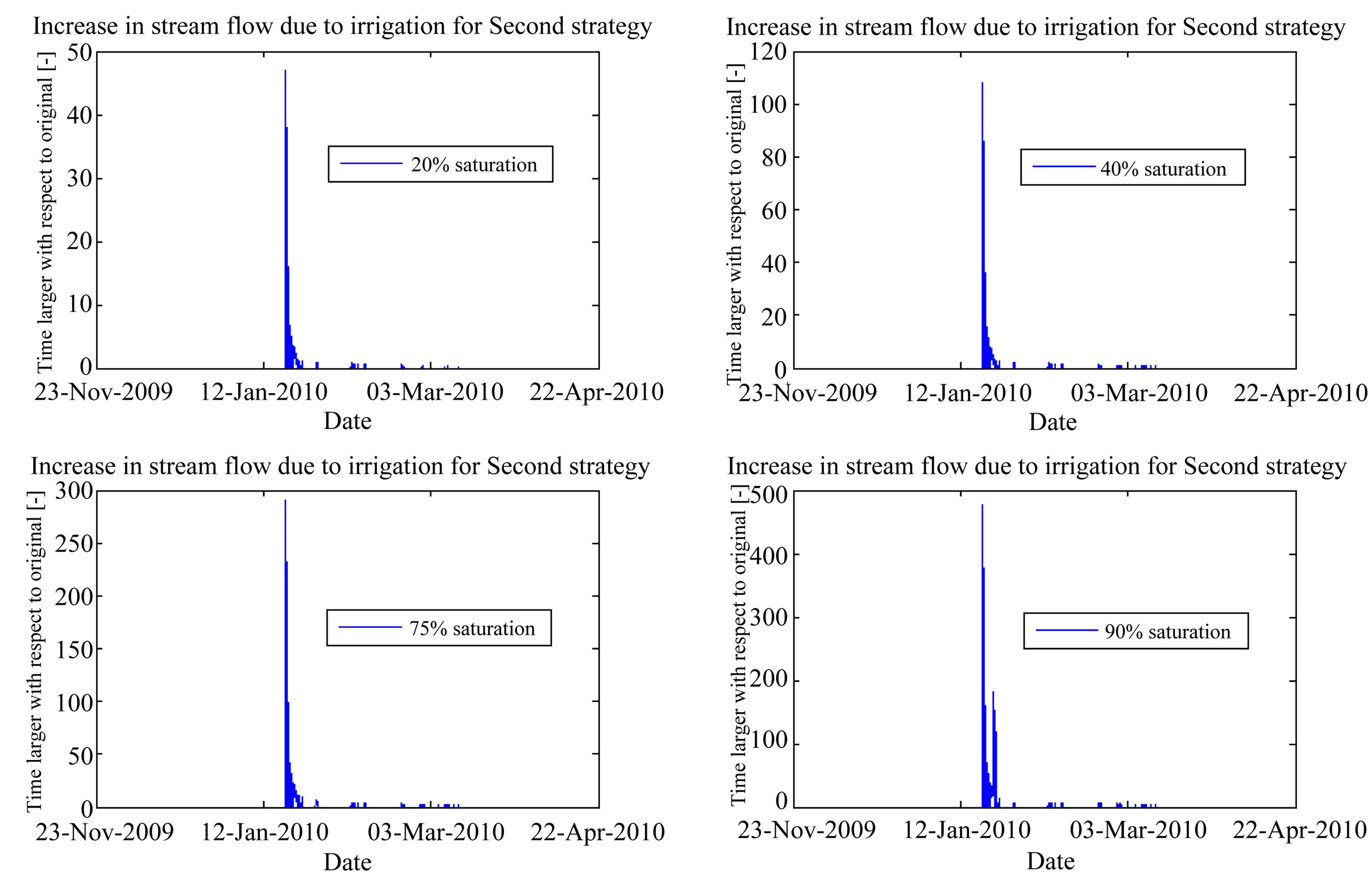
Figure 6. Relative increase in the magnitude of streamflow values for maintained soil moisture strategy.
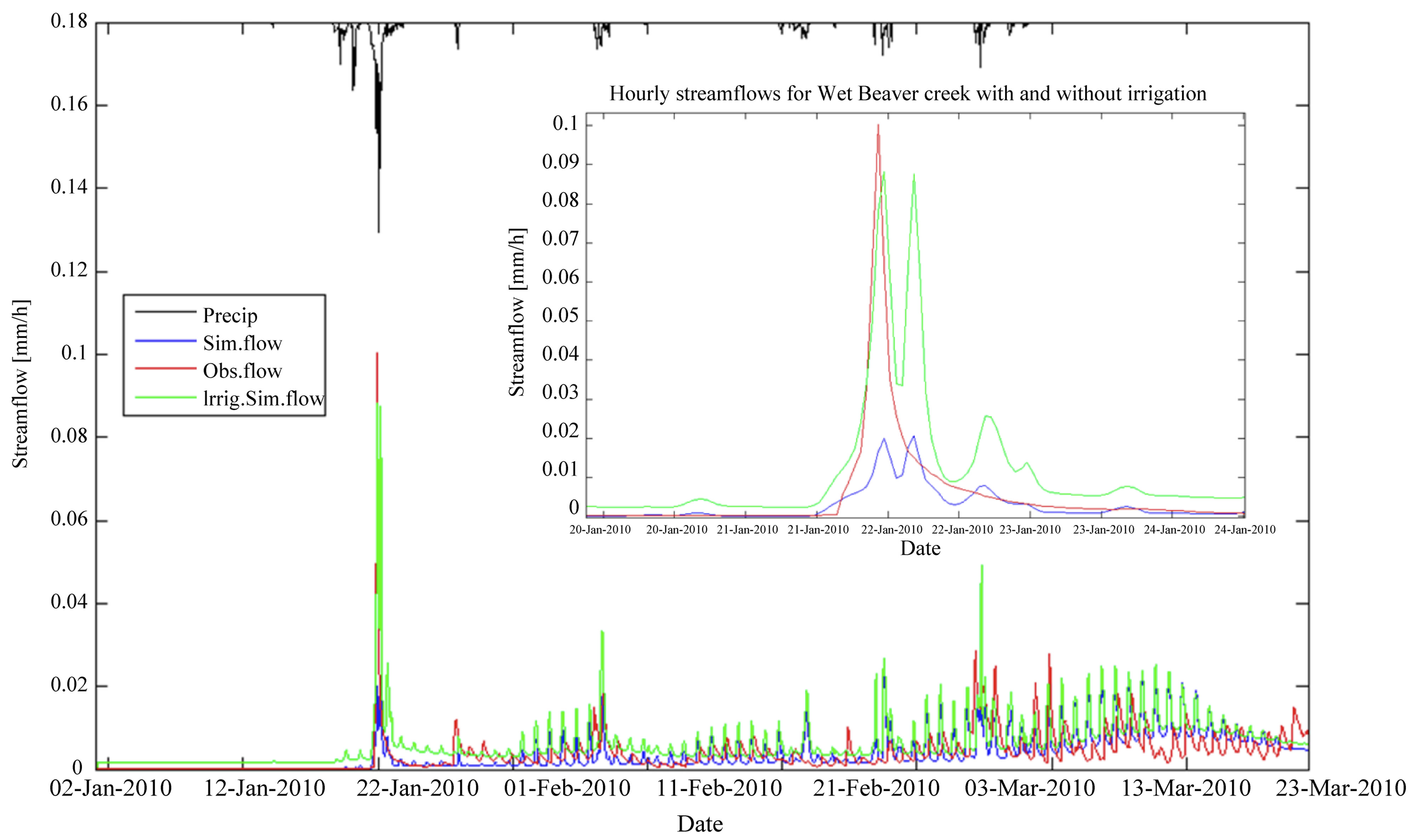
Figure 7. Simulated hydrograph for extreme case conditions (green), for non-irrigated scenario (blue), and observed hydrograph (red) in Beaver Creek. The average precipitation in the sub-basin is presented on top (in black). The flow peak for the main precipitation event on January 22nd is presented in detail in the box to the right.
soil moisture levels are maintained above the reference crop level. In the simulations that include irrigation strategies, the flood peaks produced by the main rainfall event on January 22nd increase up to two orders of magnitude compared to the original non-irrigation simulation (Figure 6), while the flow peaks produced by smaller rainfall events increase about ten times. The impact of irrigation practices on the value of peak flows is proportional to the magnitude of the precipitation event that originates them. This differential impact on flow peak magnitude can be a very useful tool for hydrograph calibration, especially when a model originally ignores the impact of irrigated lands within its area of study, and it can only calibrate well a specific range of peak flow magnitudes, but not all the values at the same time. The inclusion of irrigation strategies in the simulation process improves the calibration of flow peaks, without necessarily changing the resolution or quality of input data.
The maintaining constant soil moisture level strategy constitutes an ideal irrigation practice, since the soil gets the exact amount of water needed at every time step. In real irrigation practices, however, the farmer usually sets up a constant rate of irrigation that does not always necessarily coincides with the amount of water the soil needs, and for that reason they are not optimally effective. As irrigation rates are adjusted more often, based on soil moisture information, then real irrigation practices get closer to the optimum effectiveness achieved by maintaining soil moisture level strategy.
Reference crop level represents the optimum moisture level at which soil must be kept to grow crops: lower levels do not meet crops water demand, and higher levels waste water as baseflow, increasing the risk of flash floods during rain, because they keep water beneath the root zone where crops are not able to reach it. The effectiveness of the constant rate of irrigation strategy decreases as the soil moisture level increases, even though the total volume of water used for this strategy was the same as that for the (100% effective) maintaining constant soil moisture strategy: the latter indicates that for a farmer, to know the total amount of irrigation water for the season is not as important as how much water to use at every time step.
5. Recommendations
The rapid response of simulated hydrographs to precipitation indicates that the resolution used for the VIC model was fine enough to detect flash floods in Beaver Creek watershed. A stronger validation of hydrograph response to irrigation practices requires the evaluation of other regions with higher-quality input information, including topographic features. The following recommendations are useful to face model resolution limitations and to improve accuracy of data.
• Simulate irrigation for an entire crop cycle and add detailed field information. It is important to include harvesting times and real irrigation schedules from farmlands. Root depth and plant height should be modified in time, and not simply be constant as it is usually assumed in simulation processes.
• Consider a limited source of water for irrigation. A routing model should be modified so water channeled upstream can be directed to irrigation.
• Use explicit topography-descriptive models. To have a better understanding of the consequences associated to a flash flood event, a floodplain analysis for the sub-basin should be performed with descriptive software that offers floodplain delineation capabilities and hydrologic routing, among other features.
• Use a physical model to measure irrigation and streamflow. Flash floods have been detected in basins smaller than 1.2 km2 [19]. A basin with such dimensions can be set up within an experimental watershed, to measure all relevant variables like irrigation volumes, soil moisture, streamflow, precipitation, and detailed topography.
6. Acknowledgements
This research has been supported by the National Weather Service and SAHRA (Sustainability of Semi-Arid Hydrology and Riparian Areas) at the University of Arizona under the STC Program of the National Science Foundation, Grant No. EAR-9876800. The first author also thanks the financial support of the Lewis Delbert R. Graduate Fellowship.
REFERENCES
- S. Ashley and W. Ashley, “Flood Fatalities in the United States,” Journal of Applied Meteorology and Climatology, Vol. 47, No. 3, 2008, pp. 805-818. doi:10.1175/2007JAMC1611.1
- National Weather Service, “Definitions of Flood and Flash Flood,” 2010. http://www.srh.noaa.gov/mrx/hydro/flooddef.php
- I. Haddeland, D. Lettenmaier and T. Skaugen, “Effects of Irrigation on the Water and Energy Balances of the Colorado and Mekong River Basins,” Journal of Hydrology, Vol. 324, 1-4, 2006, pp. 210-223.
- X. L. Liang, “A Simple Hydrologically Based Model of Land Surface Water and Energy Fluxes for General Circulation Models,” Journal of Geophysical Research, Vol. 99, No. D7, 1994, pp. 415-428. doi:10.1029/94JD00483
- L. Kueppers, M. Snyder and L. Sloan, “Irrigation Cooling Effect: Regional Climate Forcing by Land-Use Change,” Geophysical Research Letters, Vol. 34, No. L03703, 2007, pp. 1-5.
- D. B. Lobell, G. Bala and P. B. Duffy, “Biogeophysical Impacts of Cropland Management Changes on Climate,” Geophysical Research Letters, Vol. 33, No. L06708, 2006, pp. 1-4.
- W. Sacks and B. Cook, “Effects of Global Irrigation on the Near-Surface Climate,” Climate Dynamics, Vol. 33, 2009, pp. 160-175. doi:10.1007/s00382-008-0445-z
- United States Department of Agriculture, “2007 Census Publications,” The Census of Agriculture, Washington DC, 2009.
- E. Todini, “The ARNO Rainfall-Runoff Model,” Journal of Hydrology, Vol. 175, No. 1-4, 1996, pp. 339-382. doi:10.1016/S0022-1694(96)80016-3
- D. R. Lohmann, “Regional Scale Hydrology: Formulation of the VIC-2L Model Coupled to a Routing Model,” Hydrological Sciences, Vol. 43, No. 1, 1998, pp. 131-141. doi:10.1080/02626669809492107
- J. Valdés, “Estimating the Impact of Soil Moisture Profiles and Its Impact in River Flow Forecasting,” National Weather Service, 2010.
- E. W. Maurer, “A Long-Term Hydrologically Based Dataset of Land Surface Fluxes and States for the Conterminous United States,” Journal of Climate, Vol. 15, No. 22, 2002, pp. 3237-3251. doi:10.1175/1520-0442(2002)015<3237:ALTHBD>2.0.CO;2
- P. Troch, “Lecture 3. Water in the Atmosphere. HWR 519. Fundamentals of Surface Water Hydrology,” Tucson, Arizona, 2010.
- G. Carbone, “Shortwave Radiation,” 2010. http://people.cas.sc.edu/carbone/modules/mods4car/shortwave/
- I. E.-N. Saeed, “Irrigation Effects on the Growth, Yield, and Water Use Efficiency of Alfalfa,” Irrigation Science, Vol. 17, No. 2, 1997, pp. 63-68. doi:10.1007/s002710050023
- J. Payero, C. Neale and J. Wright, “Near-Noon Albedo Values of Alfalfa and Tall Fescue Grass Derived from Multispectral Data,” International Journal of Remote Sensing, Vol. 27, No. 3, 2006, pp. 569-586. doi:10.1080/01431160500275713
- S. Pierce, “Alfalfa Seed Growing and Harvesting Practices in Walla Walla County, Washington,” 2002. http://www.whitman.edu/environmental_studies/WWRB/agriculture/alfalfa.html
- V. T. Chow, “Applied Hydrology,” McGraw-Hill, Inc., New York, 1998.
- G. Dick, R. Anderson and D. Sampson, “Controls on Flash Flood Magnitude and Hydrograph Shape, Upper Blue Hills Badlands, Utah,” Geology, Vol. 25, No. 1, 1997, pp. 45-48. doi:10.1130/0091-7613(1997)025<0045:COFFMA>2.3.CO;2