Journal of Water Resource and Protection
Vol.4 No.5(2012), Article ID:19464,7 pages DOI:10.4236/jwarp.2012.45027
Determining Irrigators Preferences for Water Allocation Criteria Using Conjoint Analysis
1Institute of Environmental and Water Resources Management (IPASA), University of Technology Malaysia (UTM), Skudai, Malaysia
2School of Civil and Environmental Engineering, University of New South Wales, Sydney, Australia
Email: *noorulhassan@utm.my
Received January 12, 2012; revised February 13, 2012; accepted March 16, 2012
Keywords: Conjoint Analysis; Water Allocation; Pairwise Comparison; Warabandi
ABSTRACT
Water allocation based on multiple criteria has the potential to maximize the total benefits to be gained from the use of a single unit of water. However most of the multi-criteria methods inherently include a considerable degree of subjectivity. In this study, we have attempted to reduce the subjectivity factor from water allocation decision-making process by introducing a conjoint analysis method. Opinions on the importance of a number of water allocation criteria were sought from a large number of irrigation farmers. The opinion survey data were then analyzed using the traditional conjoint analysis method which is widely used to analyze marketing surveys. The analysis allowed objective determination of the relative importance of five water allocation criteria (i.e. net farm income, percent of family working on the farm, amount paid to irrigation agency for canal water share). Each water allocation criteria was divided into three levels and utility values for each criteria level were estimated from the farmers’ preferences on five water allocation criteria (attributes). The conjoint survey results revealed that the respondents prefer that “annual net farm income” be the most important attribute in water allocation decisions. As would be expected the vast majority of the respondents overwhelmingly placed the “water price” in the last position.
1. Introduction
Today because of changing climate, high population pressures, water scarcity and increased awareness of the long term implications of excessive use of water every effort should be made to use this resource optimally to enable more production from less water [1]. Previous studies conducted in Pakistan revealed that scarce irrigation water was being allocated to inefficient farmers under the warabandi1 system, where value of a single unit of water was found very low [2,3].
The principles set in the 19th century for the design of the warabandi irrigation water delivery system in Pakistan, and notionally still being followed today are not in fact still being practiced. The farmers, with the assistance of irrigation officials have rearranged the irrigation water delivery system (warabandi) rules. The influential farmers have set their own rules to get extra water for meeting the crop-water demand of their farms [2,3]. These practiced rules favor the owners of the larger farms and those whose farms are at the upstream ends of the distributary watercourses [3]. Thus there is a need to develop a decision support system that can incorporate the needs of all farmers regarding canal water supplies, and to provide reliability and certainty of water delivery to give farmers confidence to invest in efficient water use practices. In this study a novel concept of developing improved water allocation based on multiple, farmer chosen criteria has been attempted. Given this, it is essential to know what factors or criteria the farmers consider should influence water allocation decisions so that an equitable and efficient system can be developed to improve productivity from the scarce water resource. Current productivity is very low. For example irrigated wheat production is about two tons per hectare whereas in developed countries dryland wheat cultivation typically averages more than this and irrigated yields are at least twice as high.
This paper focuses on the process of estimation of relativeness among the important water allocation criteria. This relativeness could be interpreted as a search for which criteria should be taken into consideration and which should be given little or no attention in water allocation decisions. Conjoint analysis (CA) is a technique for establishing the relative importance of different attributes (in conjoint analysis, criteria/factors are called attributes) in the provision of a service [4]. It has its origins in market research where it has been used to establish what attributes influence the demand for different commodities, and thereby what combinations of such attributes will maximize the benefits of a service. It has also been widely used in transport. Journal of Transport Economics and Policy (JTEP) published a special issue on the application of conjoint analysis method in transport [5]. Conjoint analysis has also been applied for solving environmental problems [6,7]. However, to date its application in the area of water resources management is very limited. The next section describes the conjoint analysis method and the data collection process for this study. Following this, results are presented and discussed, and conclusions are drawn concerning the relative importance of water allocation attributes.
2. Designing Conjoint Study
Conjoint analysis is a multivariate technique developed specifically to understand how respondents develop preferences for any type of object (product or service or idea). It is based on the simple principle that respondents evaluate the worth of an object by combining the separate amounts of attribute values [8]. Individuals rarely express how they do this, but relative value judgments must be made and conjoint analysis attempts to emulate this process. Conjoint analysis is unique among multivariate methods in that the researcher first constructs a set of real or hypothetical objects/profiles by combining selected levels of each attribute. Conjoint analysis, compared to other multivariate techniques, has few statistical assumptions, and accordingly, it is based on logic and pragmatism when it concerns such issues as its design, estimation, and interpretation [9].
Designing attributes, assigning attribute levels, deciding which profiles should be presented to the respondents for preference elicitation, establishing the preferences, choosing a method of profile presentation, and selecting a method for estimating utility values are the six important stages in the design of a conjoint study. These conjoint design stages within the context of a water allocation study will now be explained.
2.1. Establishing the Attributes
Water resources planning and management objective is associated with many monetary and nonmonetary attributes or criteria [10]. Decision-making for managing scarce water resource by considering all important attributes could not be possible by merely applying customary cost-benefit analysis approach as this approach can only take monetary attributes into decision analysis. Therefore, a multi-criteria analysis (MCA) approach (e.g. conjoint analysis) is required for making decisions on water resources management and planning.
It is important to say that the selection of attributes is a very important stage in a conjoint study as the final output entirely depends on the included attributes. In this study, initially ten water allocation attributes were discussed with a focus group of 20 people from an agricultural decision body in Sindh, Pakistan. These people were actively involved in farm and water management decisions as most of them were managing their own agricultural farms. Some of them were running their own agro-based businesses. The discussion with the focus group ended with the selection of the five attributes they thought to be the most important water allocation attributes for their region and these were included in this study. The attributes included were: percent of individual farmer’s family working on the farm, the amount paid annually to the Provincial Irrigation Department (PID) for canal water share, the annual net farm income, water use efficiency—i.e. the proportion of received water effectively used, and the quality of groundwater beneath the farm.
2.2. Assigning Attribute Levels
Reference [4] suggested that the attribute levels should be plausible, actionable and capable of being traded-off. In this conjoint study, the attribute levels were decided from survey data gathered from 184 farms situated in Sanghar and Shaheed Benazir Abad (formerly known as Nawabshah) districts of Sindh, Pakistan. Three levels only, were adopted, to keep survey logistics within manageable bounds. Three levels determine there are 243 (35) possible combinations. Four levels would increase this number to 1024 (45). The first and the third levels of each attribute were decided as the minimum and maximum values of that attribute obtained from the survey. For example, on the average, the minimum and maximum amounts paid annually to the PID for canal water share were found to be USD 13 and USD 25 per hectare respectively. These figures were assigned Level-1 and Level-3 for that particular attribute. The average amount paid to PID was determined as about USD 18 per hectare per year. Thus, Level-2 of that particular attribute was decided as 13 - 25 USD/ha. Levels for the other attributes were determined in the same way. The attributes and levels included in the conjoint study are shown in Table 1.
2.3. Deciding Which Profiles to Present
Having established the attributes and their levels, hypothetical profiles with different combinations of attribute levels were presented to 62 individuals (farmers). The attributes and levels chosen in this study gave rise to 243 (3 × 3 × 3 × 3 × 3) possible profiles for the water allocation problem. Obviously, it would have been imprac-
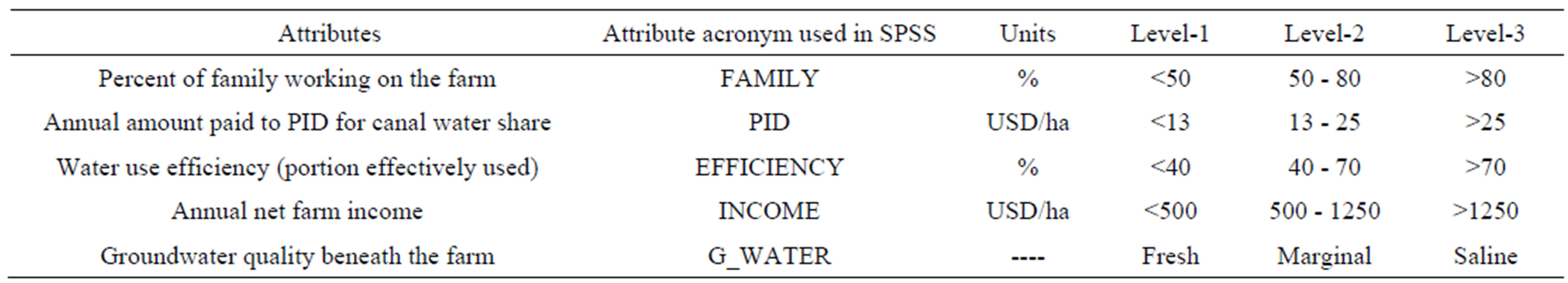
Table 1. Attributes of water allocation and their levels.
tical to ask individuals their preferences among so many profiles. Many methods exist to reduce the number of profiles to a manageable level. These include the use of fractional factorial designs; removing options that will dominate or be dominated by all other options; and dividing the possible options into blocks and establishing respondents’ preferences for a block of possible profiles. It was decided to use a fractional factorial design using the statistical package Orthoplan provided in SPSS 11.5 [11]. The use of orthogonal main-effects design reduced 243 profiles to 16. In Table 2 sixteen hypothetical profiles are shown in columns 1-6. In the last column of Table 2 the average preferences from 62 respondents are shown.
2.4. Establishing Preferences
After selection of attributes, attribute levels, and profiles, the next step was to present the profiles to the participants and to ask for their preferences. The decision on the type of preference measure to be used must be based on practical as well as conceptual issues. Many researchers favor the rank-order measure because it depicts the underlying choice process inherent in conjoint analysis. From a practical perspective, however, the effort of ranking large numbers of profiles becomes overwhelming for respondents. On the other hand, the ratings measure has the inherent advantage of being easy to administer in any type of data collection context. Because of this characteristic, a rating preference measure was selected for this study to determine the respondents’ preferences between nominated profiles. Each respondent was asked to rate their preference between two profiles on a scale from one to five (1 = no preference or rejection; 2 = weak preference; 3 = strong preference; 4 = very strong preference; 5 = absolute preference).
2.5. Choosing a Presentation Method
There are three methods by which the profiles could be presented to the respondents in a conjoint study. These presentation methods are: Trade-off, full-profile, and pairwise comparison [12]. In this study, a pairwise comparison was selected as a presentation method. But 16 profiles could produce 120 possible pairs of profiles.
In a conjoint survey, it was impractical to ask a respondent to show his preferences between 120 pairs. Thus, these 16 profiles were randomly split into two groups (8 profiles in each group). Even 8 profiles in a pair-wise comparison could generate 28 pairs. It would have been difficult for a respondent to maintain concentration while showing his preferences to 28 profile pairs. Thus, one profile was randomly selected from each group and this quasi-profile was compared with each of the remaining 7 profiles of that specific group. This resulted in 7 pairs to be compared by each respondent and was thought to be practicable within the available time and finance limitations. These two profile groups formed the basis of two separate conjoint analysis questionnaires. Sixty-two subjects (31 for each group were randomly allocated between these two questionnaires. An example of one of the pair-wise choices is shown in Figure 1. The 1 - 5 rating scale was used to show the preference for one profile relative to the other.
2.6. Selecting Method for Utility Value Estimation
Estimating the utility value for each attribute level and the relative importance of the various attributes are the two main objectives of a conjoint study. To achieve those objectives, a relationship between the attributes and utility values needs to be specified. Generally there are two types of attributes, the benefit type and the cost type. The higher the benefit type value, the better it is, and for the cost type, the opposite is true. However, for some attributes (for example, “quality of groundwater”), it was difficult to assume a linear relationship between different attribute levels prior to the actual survey (i.e. whether respondents would prefer canal water to be supplied to farms underlain by fresh or saline groundwater). Because of this difficulty, a separate utility value relationship was assumed for each of the attributes used in this study and the methodology to do this is described next.
3. Collecting and Analyzing the Data
The results from the preliminary survey regarding the ranking of ten water allocation attributes from 20 decision makers described in Section 2.1, suggested that individuals understood the questionnaire and showed their preferences in a meaningful way. However, some respondents expressed difficulties in assigning absolute
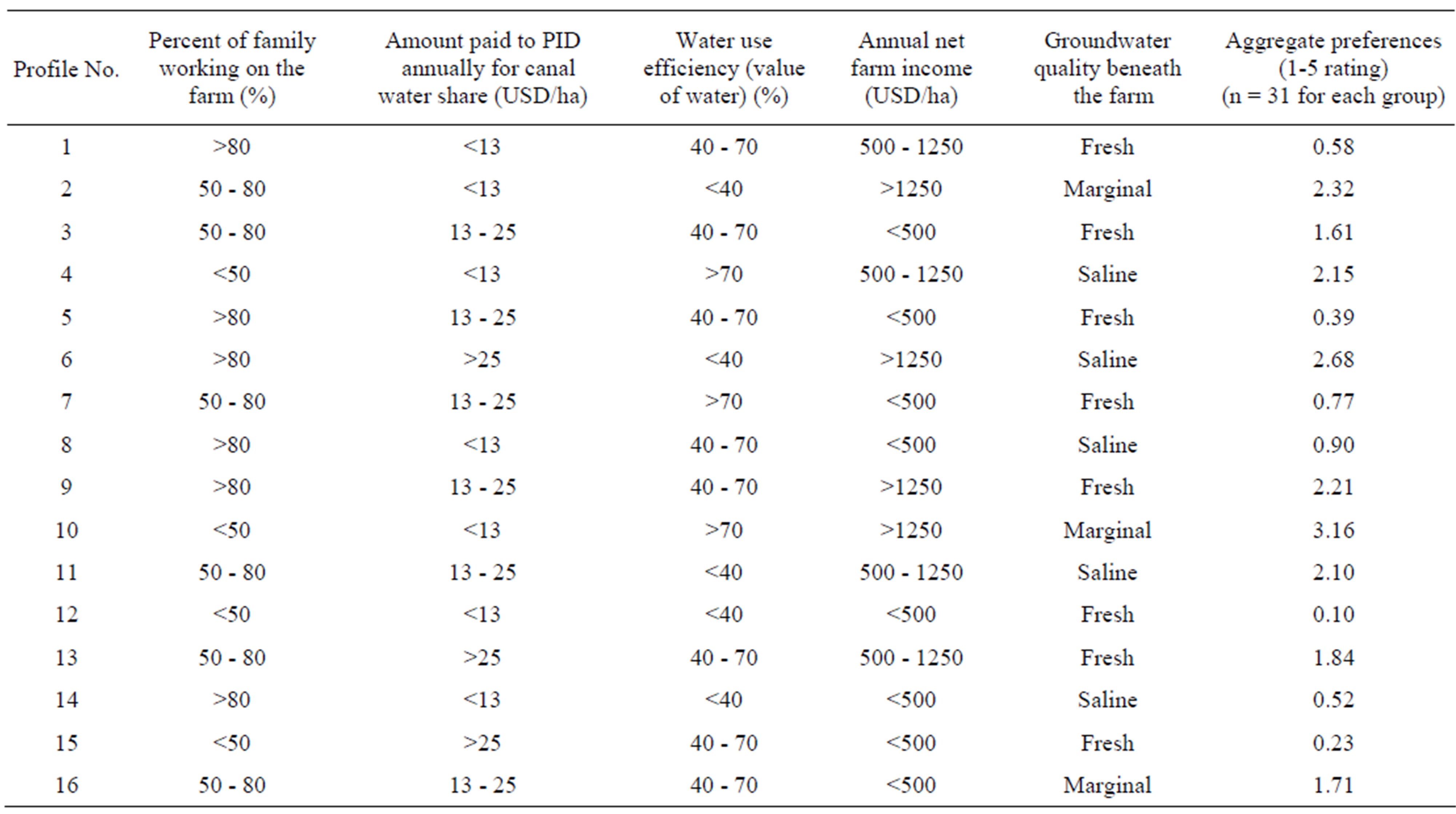
Table 2. List of adopted hypothetical profiles and aggregate preferences.
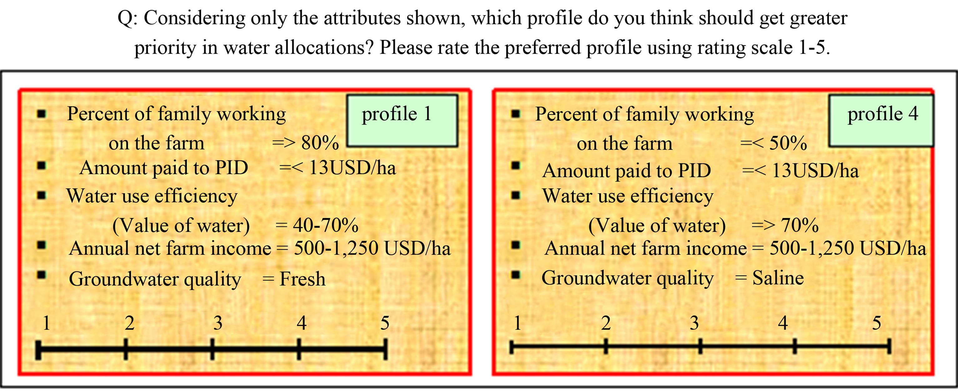
Figure 1. Example of pairwise choice to be made by participants.
rankings to the attributes and suggested that the preference scale should be flexible. Thus a rating scale of preferences was selected for the final conjoint questionnaire. Another problem faced by the survey participants was the large number of attributes they were asked to rank. In order to minimize that problem in the final conjoint questionnaire, the number of water allocation attributes included was reduced to five, as discussed above. The less important attributes were dropped from the questionnaire. The chosen water allocation attributes include: labor employed in the farming, farmers’ income, revenue generated by PID, water use efficiency, and groundwater quality beneath the agricultural farm. A face-to-face survey was conducted with 62 decision makers in the Lower Indus River Basin of Pakistan (parts of districts Sanghar and Shaheed Benazir Abad). In a pairwise comparison each respondent was asked to assign ratings to the profile he considered more deserving of receiving water. Each profile was displayed on a sample card, as shown in Figure 1, which contained one of the mixes of the levels for the five water allocation attributes shown in Table 2. Only one level of each attribute was presented in a single profile. An SPSS orthogonal sample design was used to select the particular levels to be included on each card to allow estimation over the entire range of profiles.
From the use of conjoint analysis, utility values for each of the attribute level were computed from the participants’ preferences on five water allocation attributes. These utility values along with their rank order are shown in Table 3.

Table 3. Utility value and rank order of each attribute level.
3.1. Estimation and Interpretation of Utility Values
The averages of the preference scores assigned to the sixteen profiles are shown in column 7 of Table 2. The preferences were analyzed with the conjoint procedure (available only through command syntax in SPSS 11.5 standard version) to estimate the utility values for each level of the attributes. The estimated utility values provide a quantitative measure of the preference for each attribute level, with larger values corresponding to greater preference. Utility values are expressed in a common unit, allowing them to be added together to give the total utility, or overall preference, for any combination of attribute levels. In the SPSS conjoint procedure, all attributes were assumed to be discrete data. The estimated utility values for each attribute level along with rank orders are shown in Table 3. Other things being equal, a higher utility value for a particular attribute level indicates a higher influence of that attribute on the overall preference. Figure 2 shows the trend of estimated utility values for each level of five water allocation attributes. The higher range of utility values for the “annual net farm income” attribute indicates that respondents consider this the most important attribute in water allocation decisions.
The highest utility value of 2.60 for Level-3 of “annual net farm income” attribute shown in Table 3 means that a unit increase in annual net farm income (for instance from Level-1 to Level-3) will increase the preference or utility value of “annual net farm income” by 1.82 (2.60 – 0.78). On the other hand, almost identical utility values for Level-1 of “percent of family working on the farm”
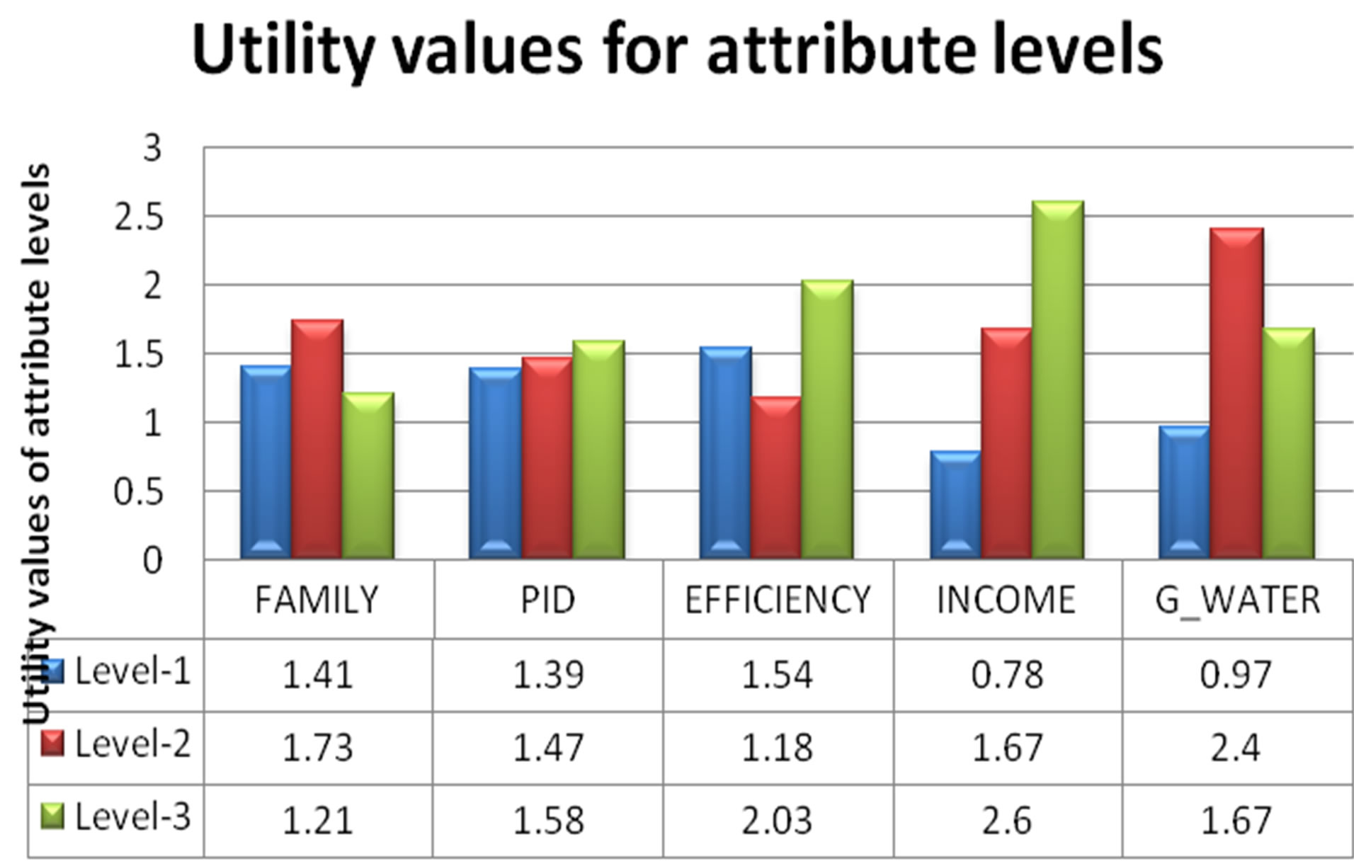
Figure 2. Estimated utility values for attribute levels.
(i.e., 1.41) and for Level-2 of “amount paid to PID for canal water share” (i.e., 1.47) suggest that the respondents were indifferent in their choice between these two levels. The large preference for “marginal” in the groundwater attribute suggests farmers are of the view those who have access to fresh groundwater are less deserving of receiving canal water than those who have no alternative supply possibilities.
3.2. Relative Importance of Attributes
As the estimated utility values are on a common scale, so the relative importance of each attribute can be computed directly. The importance of an attribute is represented by the range of its levels (i.e., the difference between the highest and lowest values of utility values) divided by the sum of the ranges across all attributes. This calculation indicates the relative impact or importance of each attribute based on the size of the range of its utility value estimates. Attributes with a larger range for their utility values have a greater impact on the calculated overall utility value and thus are deemed of greater importance. The relative importance weights across all attributes will total 100 percent. An example of how the relative importance weights for different attributes were determined is illustrated below, with reference to Table 3, for the attribute “percent of family working on the farm”. The range of utility values for FAMILY attribute was determined as 0.52 (1.73 – 1.21). The sum of ranges of utility values for all five attributes was 4.81 [(1.73 – 1.21) + (1.58 – 1.39) + (2.03 – 1.18) + (2.60 – 0.78) + (2.40 – 0.97)]. The range of utility values for FAMILY attribute (0.52) divided by the sum of ranges of utility values for all attributes (4.81) gives the relative importance weight of 10.8% for this particular attribute. The relative importance weights for the remaining attributes were similarly determined and are plotted on Figure 3.
4. Overview of Conjoint Results
From the relative importance weights for each attribute, it can be seen that the respondents gave more importance (37.8%) to the “net farm income” attribute than to other water allocation attributes. This means the respondents preferred to allocate water to those who would make the highest income from it. The respondents considered “groundwater quality beneath the farm” the second most important water allocation attribute with relative importance of 29.7% followed by the “irrigation water use efficiency” (17.7%). The least important attribute with relative importance weight of merely 4.0% was “amount paid to PID”. Though it appears individuals were more willing to improve water use efficiency than to engage more family members in the farming enterprise (Figure 3), there is some ambivalence as can be seen from the conflicting, or inconsistent utility values shown in Table 3 for these attributes. Comparing the groundwater quality attribute with the remaining water allocation attributes, the respondents prefer water allocations to go to the less
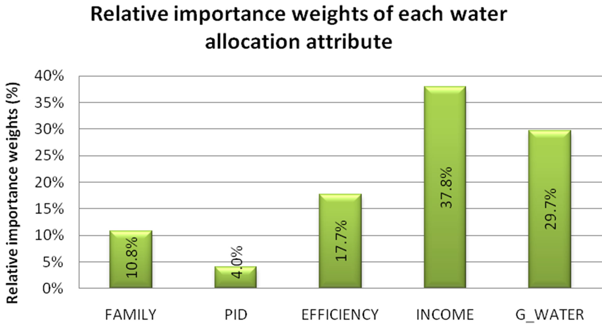
Figure 3. Relative importance weights for water allocation attributes.
efficient water users (1.18) and the districts where a very small charge was paid to PID for water supplies (1.39) rather than to the areas where “fresh” groundwater (0.97) was available. This preference clearly indicates that measurable economic or environmental benefits are not necessarily dominant in the thinking of these water users. Some compassion is apparently important, in this case for those who have no alternative means of obtaining crop water other than from the canal supply.
If the farmers were asked to choose one from two options of either: to raise their farm income from the existing income of <500 USD/ha to >1250 USD/ha or to increase the numbers of their family members working on the farm from <50% to >80%, the farmers would be about four times as attracted to raise the net farm income than to put more family members into farming—as the utility value difference between two extreme levels of net farm income was 1.82 (2.60 – 0.78) and the utility value difference between lowest and the highest levels of “percent of family working on farm” attribute was only 0.52 (1.73 – 1.21). The conjoint analysis findings indicate that when rating the alternative water allocation profiles, within attributes the respondents attached the highest value to the “>1250 USD/ha” level of farm income (utility value = 2.60), “marginal” quality groundwater (utility value = 2.40), “>70%” of water use efficiency (utility value = 2.03), “50% - 80%” proportion of family working on the farm (utility value = 1.73), and “saline” groundwater quality (utility value = 1.67). Thus, the total utility of an ideal agricultural farm would be: U = 1.73 + 1.58 + 2.03 + 2.60 + 2.40 = 10.34.
It is interesting to note in Figure 2 and Table 3 that for three of the five attributes respondents preferred the last level (level-3) rather than either Level-1 or Level-2, which would have indicated a trend and a preference for an increase or decrease for that attribute. On the other hand, farmers preferred Level-2 of two attributes (i.e. “percent of family working on the farm” and “farms with marginal quality groundwater”). It is suggested the preference for the middle level may indicate respondents considered the “extreme” levels, which were the maximum or minimum values obtained in an earlier, larger survey, to be generally unrealistic, or unattainable to them. So being realists they voted for what they considered attainable. In the case of INCOME everyone would like increased income and so the upper extreme was preferred—perhaps in an aspirational sense.
5. Concluding Comments
In water resources management, the application of conjoint analysis to determining the importance of different attributes in deciding priorities for allocation of irrigation water is an innovative approach. From a survey of 184 farms five water allocation attributes were determined to be the most important in the thinking of the farmers. The levels or relative property characteristics of each of these five attributes were also decided from the large survey, which was conducted in the Lower Indus Valley of Pakistan. Sixty-two respondents participated in a conjoint analysis questionnaire and showed their preferences for particular farm scenarios based on nominated levels of the five water allocation attributes. The conjoint data analysis revealed that the respondents were more attracted to the “net farm income” attribute (relative importance weight = 37.8%) than any of other attributes. Quality of groundwater was second preference with relative importance weight of 29.7%. Here respondents preferred to provide canal water to those in marginal quality groundwater regions, presumably thinking those with no alternate irrigation water source were more deserving of an allocation of fresh canal water than those who had some access to an alternate (but much more expensive) freshwater supply. Not surprisingly “amount paid to the water provider” (considered as a tax) was assigned the lowest preference (merely 4.0% of relative importance weight).
While the study results cannot be considered to give definitive guidance on how water should be allocated in the Indus Valley, due to the limited range of attributes and numbers of participants included in the study, it does show that there could be an important place for conjoint analysis in objectively determining priorities in the redefining of water allocation guidelines and in the making of wider water resources decisions.
6. Acknowledgements
The authors would like to thank Ministry of Education, Government of Pakistan for the financial support provided to the first author. Partial funding was provided by Higher Education Commission (HEC) of Pakistan and the University of Technology Malaysia (under Vot No. 00L15). Special thanks are given to HEC and the UTM for their partial financial support.
REFERENCES
- R. Ali, J. Byrne and T. Slaven, “Modelling Irrigation and Salinity Management Strategies in the Ord Irrigation Area,” Natural Resources, Vol. 1, 2010, pp. 34-56. doi:10.4236/nr.2010.11005
- D. J. Bandaragoda, “Institutional Conditions for Effective Water Delivery and Irrigation Scheduling in Large Gravity Systems: Evidence from Pakistan,” Proceedings of the ICID/FAO Workshop on Irrigation Scheduling, Rome, Italy, 1996.
- N. H. Zardari and I. Cordery, “Water Productivity in a Rigid Irrigation Delivery System,” Water Resources Management, Vol. 23, No. 6, 2009, pp. 1025-1040. doi:10.1007/s11269-008-9312-2
- M. V. Pol and M. Ryan, “Using Conjoint Analysis to Establish Consumer Preferences for Fruit and Vegetables,” British Food Journal, Vol. 98, No. 8, 1996, pp. 5-12. doi:10.1108/00070709610150879
- JTEP, Journal of Transport Economics and Policy, Vol. 22, Special Issue, 1988.
- W. H. Desvousges, V. K. Smith and M. P. McGivney, “A Comparison of Alternative Approaches for Estimating Recreation and Related Benefits of Water Quality Improvements,” Office of Policy Analysis, US Environmental Protection Agency, Washington DC, 1983.
- J. Opaluch, S. Swallow, T. Weaver, C. Wessels and D. Wichelns, “Evaluating Impacts from Noxious Facilities: Including Public Preferences in Current Sitting Mechanisms,” Journal of Environmental Economics and Management, Vol. 24, No. 1, 1993, pp. 59-67. doi:10.1006/jeem.1993.1003
- J. Hair, R. Anderson, R. Tatham and W. Black, “Multivariate Data Analysis,” 6th Edition, Pearson Prentice Hall, 2006.
- J. Hair, R. Anderson, R. Tatham and W. Black, “Multivariate Data Analysis with Readings,” 5th Edition, Pearson Prentice Hall, 1998.
- D. G. Regulwar and J. B. Gurav, “Fuzzy Approach Based Management Model for Irrigation Planning,” Journal of Water Resource and Protection, Vol. 2, No. 6, 2010, pp. 545-554. doi:10.4236/jwarp.2010.26062
- SPSS Inc., “SPSS 11.5 for Windows,” Chicago, USA, 2002.
- B. K. Orme, “Getting Started with Conjoint Analysis: Strategies for Product Design and Pricing Research,” Research Publishers, LLC, Madison, 2005.
NOTES
*Corresponding author.
1Warabandi is a rotational method for equitable distribution of the available water in an irrigation system by turns fixed according to a predetermined schedule specifying the day, time and duration of supply to each irrigator in proportion to the size of his landholding in the outlet command.