Journal of Water Resource and Protection
Vol. 2 No. 11 (2010) , Article ID: 3184 , 11 pages DOI:10.4236/jwarp.2010.211110
Measuring Ice Thicknesses along the Red River in Canada Using RADARSAT-2 Satellite Imagery
Government of Manitoba, Department of Water Stewardship, Saulteaux Crescent, Winnipeg, Manitoba, Canada
E-mail: Karl-Erich.Lindenschmidt@gov.mb.ca
Received September 3, 2010; revised October 26, 2010; accepted November 4, 2010
Keywords: ice jams, RADARSAT-2, Red River, river ice thickness, snow cover depth
ABSTRACT
The spring flood of 2009 in the Red River Valley was exacerbated with severe ice breakup and ice jamming. To assist ice jam mitigation by cutting and breaking up the river ice cover before the flood season and to support the operation of the Red River Floodway, Manitoba Water Stewardship is striving to model the occurrence of ice breakup and simulate the behaviour of ice jamming along the river. An important parameter in ice breakup forecasting is the ice thickness. RADARSAT-2 standard satellite images were collected along the course of the Red River in Manitoba during the 2009-2010 winter to help determine ice thicknesses along the river. Standard images can have transmit-receive polarizations in the horizontal-horizontal (HH) or horizontal-vertical (HV) configurations. Ice thickness measurements were taken in the field during the same time frame when the satellite passed over the Red River Valley. Good correlations were obtained between the HH-backscatter readings and the surveyed ice thicknesses. HV-backscatter readings correlate better with fresh snow depth measurements. Additionally, using same sensor incident angle and flight geometry allows ice thickening rate behavior over the course of the winter to be determined.
1. Introduction
Red River spring floods are accompanied by ice jams which impact many areas along the river. Since historical times, this has been a regular phenomena, however analyses of recorded data over the past one hundred years suggests that ice jamming has become more severe within that time frame and that this state will be maintained or even be exacerbated in the near future. For instance in the past 15 years, there is an increase in the number of reported ice jams along the Red River in the United States recorded in the US Army Corps of Engineers (USACE) Cold Regions Research and Engineering Laboratory (CRREL) database (see Figure 1).
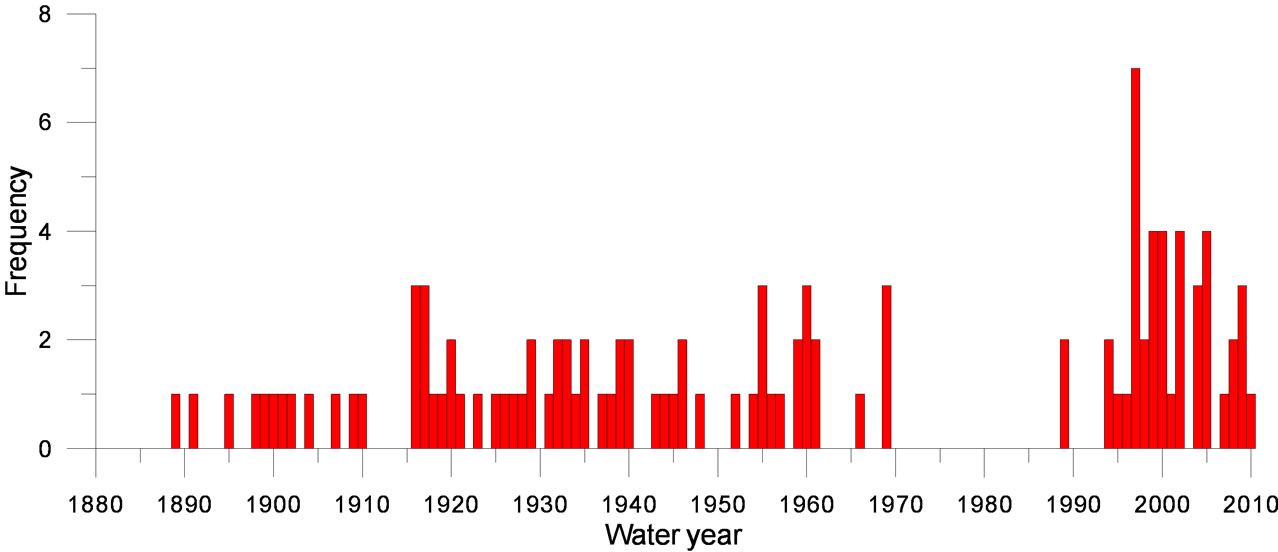
Figure 1. Number of reported ice jams along the Red River in North Dakota and Minnesota (source: https://rsgis.crrel. usace.army.mil/icejam/ accessed 9 August 2010).
Ice conditions impose challenges to the operation of the Red River Floodway, a channel circling the east side of Winnipeg to divert floodwaters from the Red River south of the city back into the Red River north of the city. The start of operation of the Red River Floodway usually occurs when the ice has broken up and a large degree of it is cleared from the Red River south of Winnipeg. If ice enters the Floodway channel it could jam against bridges and reduce channel capacity. There is evidence that ice breakup is occurring earlier in the spring. Since the Floodway was constructed in the late sixties, there is a significant trend to earlier start dates during the years of Floodway operation, approximately half a day each year (see Figure 2). This implies that breakup is now occurring tendentially three weeks earlier than when the Floodway first began operating. Ice thicknesses have not significantly decreased during this timeframe (data not shown). Earlier breakup dates along the Red River has also been confirmed by [1].
In addition, the spring freshet is occurring earlier in the year, as indicated in Figure 3. The trend in the northward migration of the 0℃ isotherm in spring [1,2] causes the snowmelt in the Red River’s headwaters to generally occur earlier and hence, supply earlier flood runoff in the northern, downstream stretches of the river in Manitoba. This leads to an earlier ice breakup downstream and there is less time for thermal processes to degrade the ice cover before ice breakup and jamming sets in. The rise in the hydrographs in the past decade has also, on average, increased sharply compared to previous decades. Increasing the strain rate of ice, due to a more rapid water level increase, makes ice more resistant to stress [3] and its fracture behaviour more brittle [4]. Increasing strength and resistance to breakup makes the occurrence of ice jamming more probable and severe.
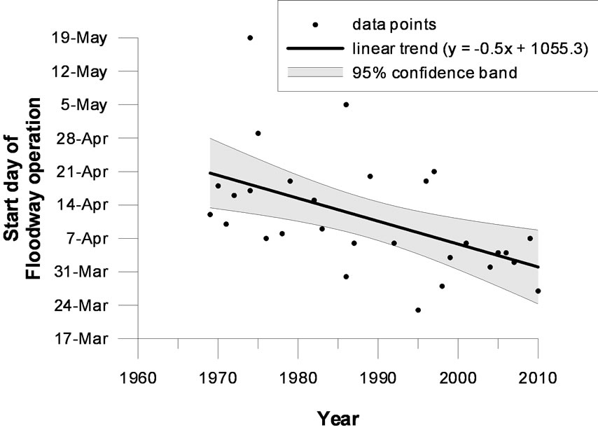
Figure 2. Decreasing trend in start dates of the years of Floodway operation.
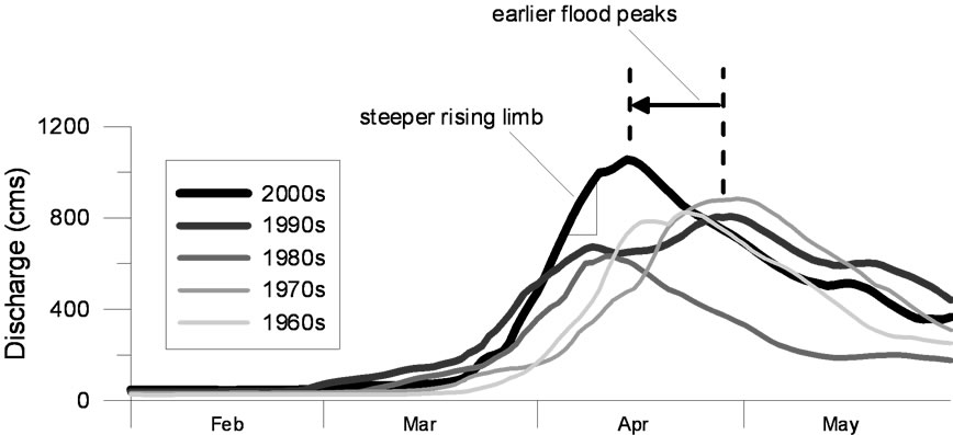
Figure 3. Discharge at Ste. Agathe averaged over 10 years for each day of the year during spring flooding (data source: Water Survey of Canada).
Hence, computer models are being developed and implemented by Manitoba Water Stewardship to predict the locations and time periods of ice breakup along the river and simulate the behaviour of resulting ice jams. Ice thickness is an important input parameter for these models, however measuring ice thicknesses on a large scale along the entire course of the river is very resource intensive. Hence, this study was undertaken to assess the potential of Canada’s RADARSAT-2 satellite to map ice thicknesses along the Red River.
Much work has been carried out to delineate river ice and classify river ice types on several rivers, e.g. along the Mississippi, Missouri and Red Lake rivers [5], Peace River [6], Saint-Francois River [7] and Athabasca River [8]. Surface texture was also included in the classification of ice along the Peace River [9]. The ice characterisation was carried out using imagery acquired by RADARSAT-1, a satellite sensor that sends and receives microwaves in a horizontal polarization mode. Attempts were also made to correlate RADARSAT-1 backscatter signals with ice thicknesses, in particular for the Peace River [10] and Athabasca River [11]. RADARSAT-2, which was launched in December 2007, provides additional technical improvements for ice characterisation over its predecessor RADARSAT-1. The new generation RADARSAT satellite can send and receive microwaves in both horizontal and vertical polarisation modes (explained in more detail below), which provides opportunities to extract additional information about the ice cover. Classification of ice types has already been investigated along the Mackenzie River [12]. The research presented here extends the methodology to include correlations of RADARSAT-2 multi-polarization backscatter signals with thicknesses of ice and snow along the ice cover of the Red River.
2. Study Site
The Red River originates along the North and South Dakota borders. It flows northward to constitute the border between Minnesota and North Dakota before continuing into Manitoba through the City of Winnipeg and onward to discharge into Lake Winnipeg (see Figure 4). The river is approximately 885 km in length with a maximum relief of 70 m and is situated in the cold continental climate zone of the Great Plains.
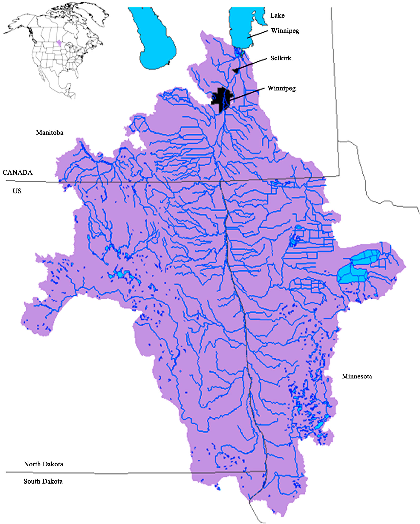
Figure 4. The Red River and its tributaries within the basin (source: Red River Basin Disaster Information Network http://www.rrbdin.org).
The Red River flows across a flat ancient glacial lakebed created at the end of the last ice age. Sediments precipitating from the melt waters during the recession of the continental Laurentide ice sheet formed the clayey lacustrine soils of the valley. The lower reach of the river is remarkably flat with a gradient of about 1:5000. Flood waters quickly overtop the banks and spread across the old lakebed. Rains or melting snow on saturated or frozen soil has caused a number of catastrophic floods, which are exacerbated by the fact that snowmelt runoff starts in the warmer south and flows northward. This frequently causes mechanical ice breakup and jamming aggravating spring flooding, especially during early and rapid melt events.
Ice on the Red River and its tributaries is typically present from November to April. The ice cover is generally smooth, and once formed, tends to remain in place through the entire winter. Flows are generally low during the winter, while ice growth appears to depend on latitude. Under normal winter conditions, ice thicknesses range from about 45 cm in the southern portion of the basin to about 75 cm near the US/Canada border to thicknesses of up to 1 m in the Winnipeg region. Breakup is triggered by snowmelt and warmer temperatures and the most severe ice jams occur north of Winnipeg.
Ice jamming occurs within Winnipeg, as well. In the extreme flood years of 1997 and 2009, ice remained largely stationary or in large pans much longer than in other years. Floodwater diversion was required before the ice was cleared to protect property in Winnipeg. Large ice pans did move into the Floodway during both events causing ice accumulations at the first bridge crossing the diversion channel. The accumulation persisted for only eight hours during the 1997 event. However, the accumulation at the same bridge during the 2009 event required mechanical removal of the ice floes using 15 extended-reach excavators for a continual period of three days before the ice cleared the channel.
3. Methodology
Radar is a ranging or distance measuring device [13]. It consists of a transmitter, a receiver, an antenna, and an electronics system to process and record the data. Referring to Figure 5 [left], the transmitter generates successive short bursts, or pulses, of microwave (A) at regular intervals which are focused by the antenna into a beam (B) at an incident angle q. The radar beam illuminates the surface obliquely at a right angle to the motion of the satellite. The antenna receives a portion of the transmitted energy reflected, or backscattered, from various objects within the illuminated beam (C).
By measuring the time delay between the transmission of a pulse and the reception of the backscattered echo from different targets, their location and characteristics can be determined. As the satellite moves forward, recording and processing of the backscattered signals builds up a two-dimensional image of the surface (Figure 5 [right]). For greater detail, the reader is referred to [13].
RADARSAT-2 operates in the C-band microwave frequency range of the electromagnetic spectrum, hence wave frequencies vary between 4 and 8 GHz (wavelengths 3.75 to 7.5 cm) [13]. At these frequencies the depth of wave penetration through the ice is potentially up to 10 to 100 m [14], hence microwaves will penetrate through the entire ice cover of the Red River. The interaction of microwaves with the river ice cover is dependent on the dielectric properties of the snow and ice, conveniently described by the value of the dielectric constant. This constant varies little with wave frequency or ice temperature for freshwater ice [15] (unlike sea ice as described in [16]), but is more affected by the water content of the overlying snow [11].
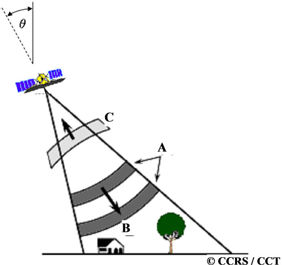
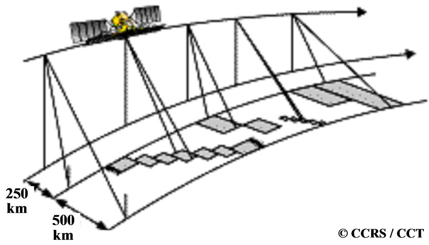
Figure 5. Radar beam transmitter from and received by the satellite [left]; construction of 2-D images from scanning sensor along the course of the satellite flight path (source: Canada Centre for Remote Sensing [13], http://www.ccrs.nrcan.gc.ca/resource/tutor/fundam/pdf/ fundamentals_e.pdf).
Surface scatter from ice is a result of the reflection which occurs when a radar signal contacts the ice cover (Figure 6 [A]). Volume scattering occurs when the radar signal penetrates the surface and is scattered within the ice sheet (Figure 6 [B]).
In standard mode the RADARSAT-2 sensor is designed to transmit microwave radiation that is horizontally (H) polarized and to receive backscattered waves that are either horizontally or vertically (V) polarized. In this mode there are two combinations of transmit and receive polarizations:
HH - for horizontal transmit and horizontal receive (copolarized)
HV - for horizontal transmit and vertical receive (crosspolarized)
The analysis of the two polarizations allows different information about the ice cover characteristics to be extracted. Cross-polarization (HV) may better detect finer features in the ice cover than with a co-polarization (HH) configuration [15]. For example in [17], better contrast between level ice and ice ridges using cross-polarization than co-polarization was attained.
The angle and profile of the transmitted beam can be adjusted so that the beam intercepts the earth’s surface over a desired range of incident angles. In this study, it was important to obtain a large coverage along the length of the Red River with one acquired image. A fixed cost per image determines pricing. In addition, increasing spatial extent is obtained at the expense of spatial resolution. Hence, the standard mode (S) was the best balance between spatial extent, spatial resolution and budget restraints (the reader is referred to [18] for a more detailed description on beam modes). The standard mode provided images covering a 100 × 100 km area with a spatial resolution of at least 25 × 25 m at a cost of CDN $300/image. The company C-Core (http://www.c-core. ca/) processed and delivered the images.
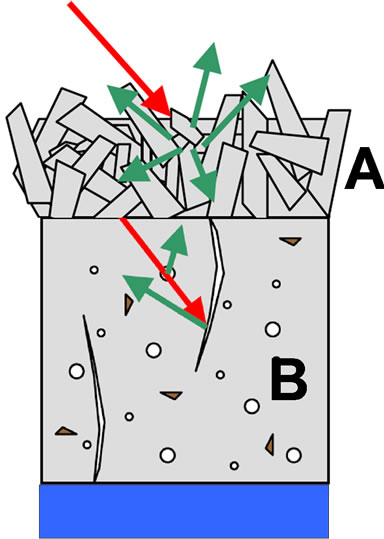
Figure 6. A: Ice texture affects surface scatter. B: Impurities and cracks cause volume scattering (modified from [11]).
Different standard mode scenes corresponding to the RADARSAT-2 flight path were available (see Figure 7). Standard mode numbers correspond to a particular incident sensor angle normal to the earth’s surface. S1 corresponds to the smallest incident angle range (20° - 27°) and S7 to the largest incident angle range (45° - 49°). The image provider obtains the best results in ice characterization using the S4, S5 or S6 modes (pers. comm.). Due to the north-south orientation of the Red River, which complies approximately with the flight orientation of the satellite, only one scene was required to capture the whole study site. The flight paths repeat themselves every 24 days. Standard No. 6 descending flight path images (S6D, incident angle ranges between 41° and 46°) were acquired for the following dates: 24-December- 2009, 17-January-2010, 10-February-2010 and 6-March- 2010.
This study was focused on the most downstream reach of the Red River between Ste. Agathe and Lake Winnipeg (see white box in Figure 7). Ten transects were chosen to carry out ice thickness and snow depth measurements, indicated in Figure 8 with station numbers accompanying station names. Three to five evenly spaced holes were drilled into the ice across each transect spaced 25 or 50 m apart, depending on the width of the river at each transect. Surveys were carried out in 2010 on 18 + 19 January, 10 + 11 February and 8 + 9 March to coincide with the approximate times of satellite image acquisitions. A survey was not carried out in December due to work safety considerations stemming from the low ice thicknesses. Stations were chosen to provide ice thickness measurements for a wide range of backscatter values. At times, these locations were conveniently in close proximity to each other. Hence, some stations appear to be paired to reduce the time and effort of the survey program. Stations were not chosen in urban areas due to potential dangers of thin ice caused by discharge outfalls.
4. Results and Discussion
RADARSAT-2 images were acquired of the Red River between Ste. Agathe and Lake Winnipeg during winter 2009 – 2010. An extract of these images is provided in Figure 9 and Figure 10 for the river stretch between St. Adolphe and southern Winnipeg. This extract includes the transect stations #5 and #6. Figure 9 is the backscatter received using the HH, Figure 10 for the HV transmit-receive configuration.
The backscatter from both HH and HV configurations where lowest in December, when the ice is thinnest and there is the least snow accumulation on the ice cover during the course of the winter. The increase in measured backscatter is the most prevalent for the first 24 day interval between 24. December 2009 and 17. January 2010.
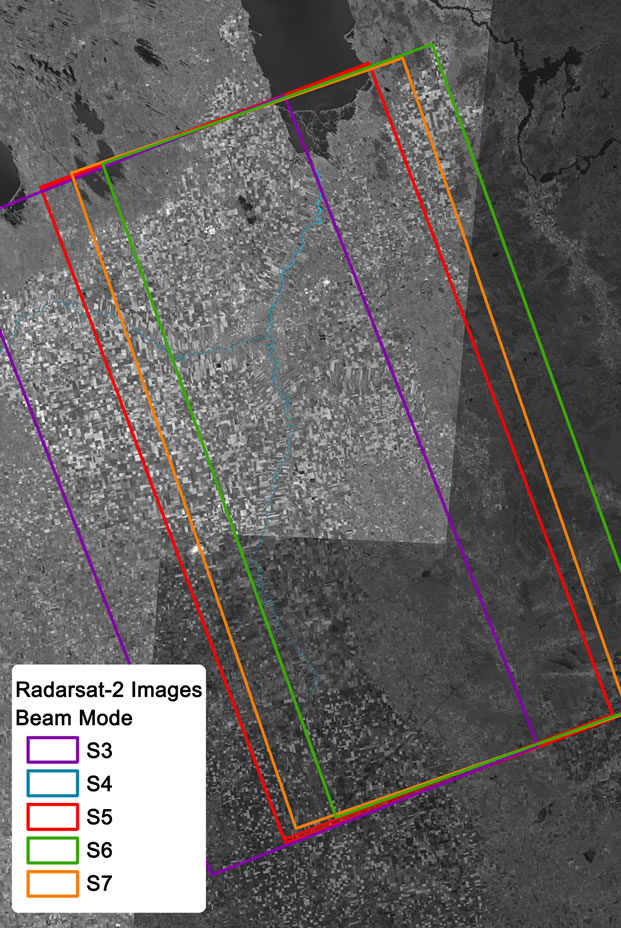
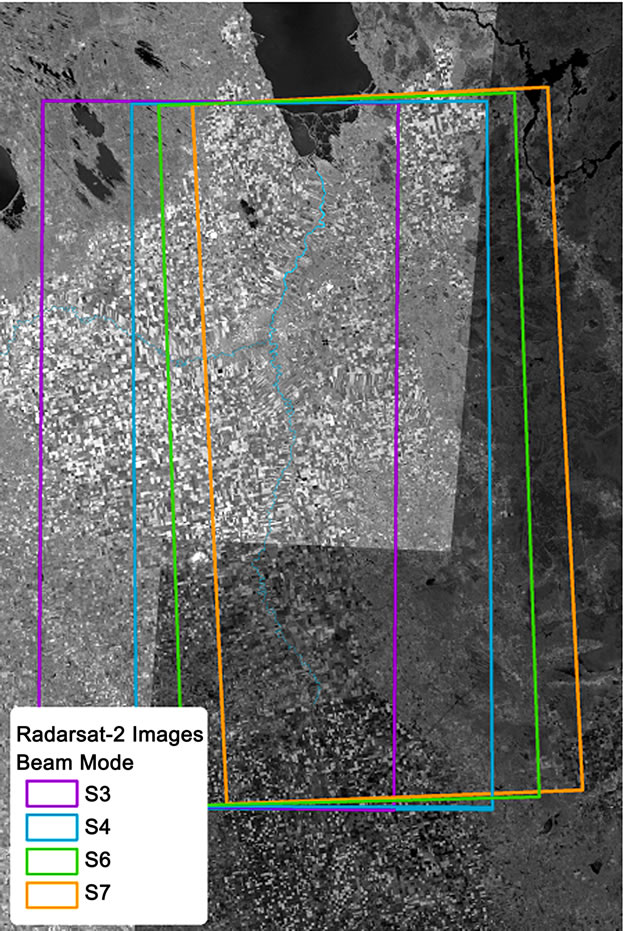
Figure 7. Standard scenes of the RADARSAT-2 flight path over the Red River Valley, both for ascending (left panel) and descending (right panel) flights (source: C-Core, http://www.c-core.ca/). The white box indicates the study area.
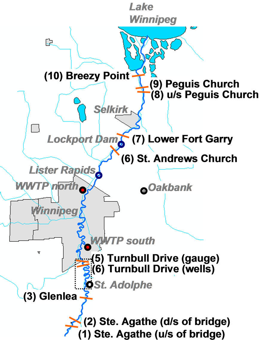
Figure 8. Most downstream reach of the Red River between Ste. Agathe and Lake Winnipeg. Station names and numbers (black normal text) indicate location of ice thickness and snow depth measurements for ground-truthing of satellite imagery (u/s = upstream; d/s = downstream). Additional place names (gray italicized text) are referred to in the manuscript and provided for orientation. Dotted box indicates zoomed area for Figure 9 and Figure 10.
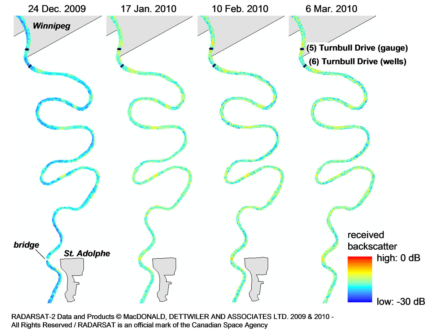
Figure 9. Backscatter images between St. Adolphe and Winnipeg acquired using the HH polarization. Image acquired using the S6D sensor configuration at 24 day intervals during winter 2009-2010. Zoomed area is indicated in Figure 8.
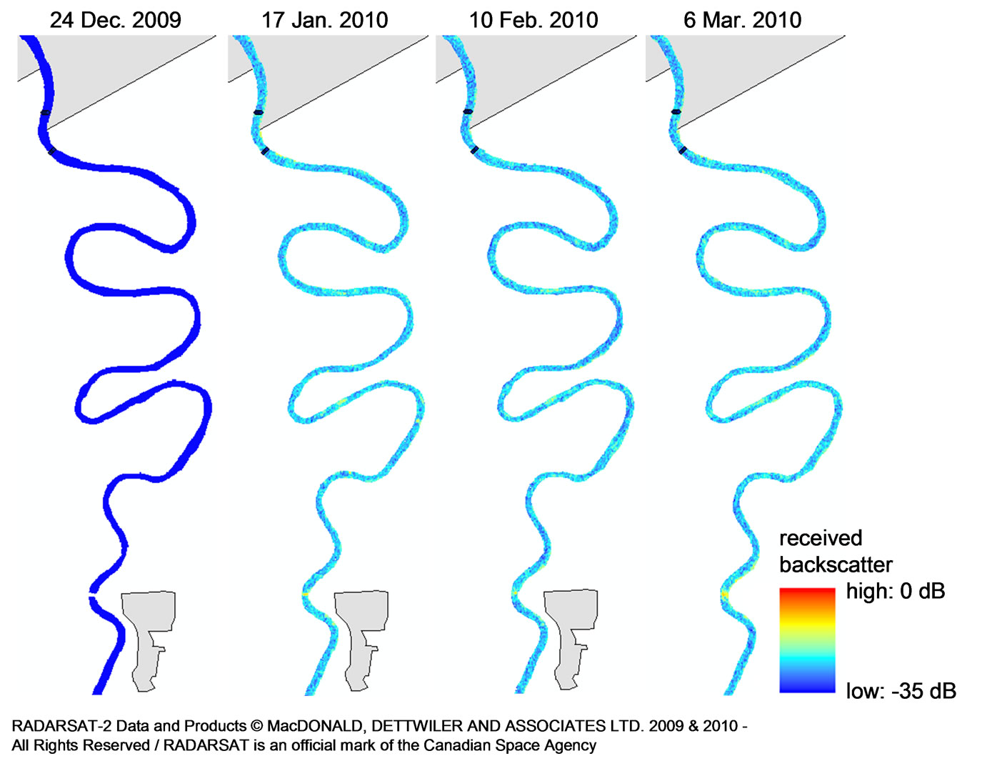
Figure 10. Backscatter images between St. Adolphe and Winnipeg acquired using the HV polarization. Image acquired using the S6D sensor configuration at 24 day intervals during winter 2009-2010. Zoomed area is indicated in Figure 8.
Backscatter signals are generally weaker for HV compared to HH.
Figure 11 shows the longitudinal profile of the HH readings along the Red River from the March 2010 acquired image. The mean µ, standard deviation s and maximum and minimum values (max and min) were determined in ArcGIS using a window of radius 50 m moved every 50 m along the river centerline. The range of the ± 1 standard deviation (± 1 s) from the mean and the total extent of the values (max/min) are represented with dark and light shading, respectively. The scatter in the values, represented by the ± 1 s and max/min ranges, indicated the high spatial heterogeneity of the signal readings, even pixels in close proximity to each other.
Ice thickness measurements correlated best with HH readings and are superimposed on the HH longitudinal profiles from 6. March 2010 in Figure 11. Ice thicknesses, too, are very heterogeneous, even along the same transect. The largest difference in the measurements was at St. Andrew’s Church, with ice thicknesses differing by 265 mm across the transect (ranging between 495 and 760 mm).
Due to the heterogeneity in both data sets, the backscattered signals and the ice thickness measurements, it was deemed best to make correlations between the mean values of the two data sets at each transect. This is a similar approach adapted by [11]. HH backscatter and ice thicknesses correlate well especially as the winter progresses into March (see Figure 12) when the coefficient of determination r2 improved from r2 = 0.43 for January to r2 ≈ 0.60 for February and March. An increase in the correlation was also obtained by [11] for the Athabasca
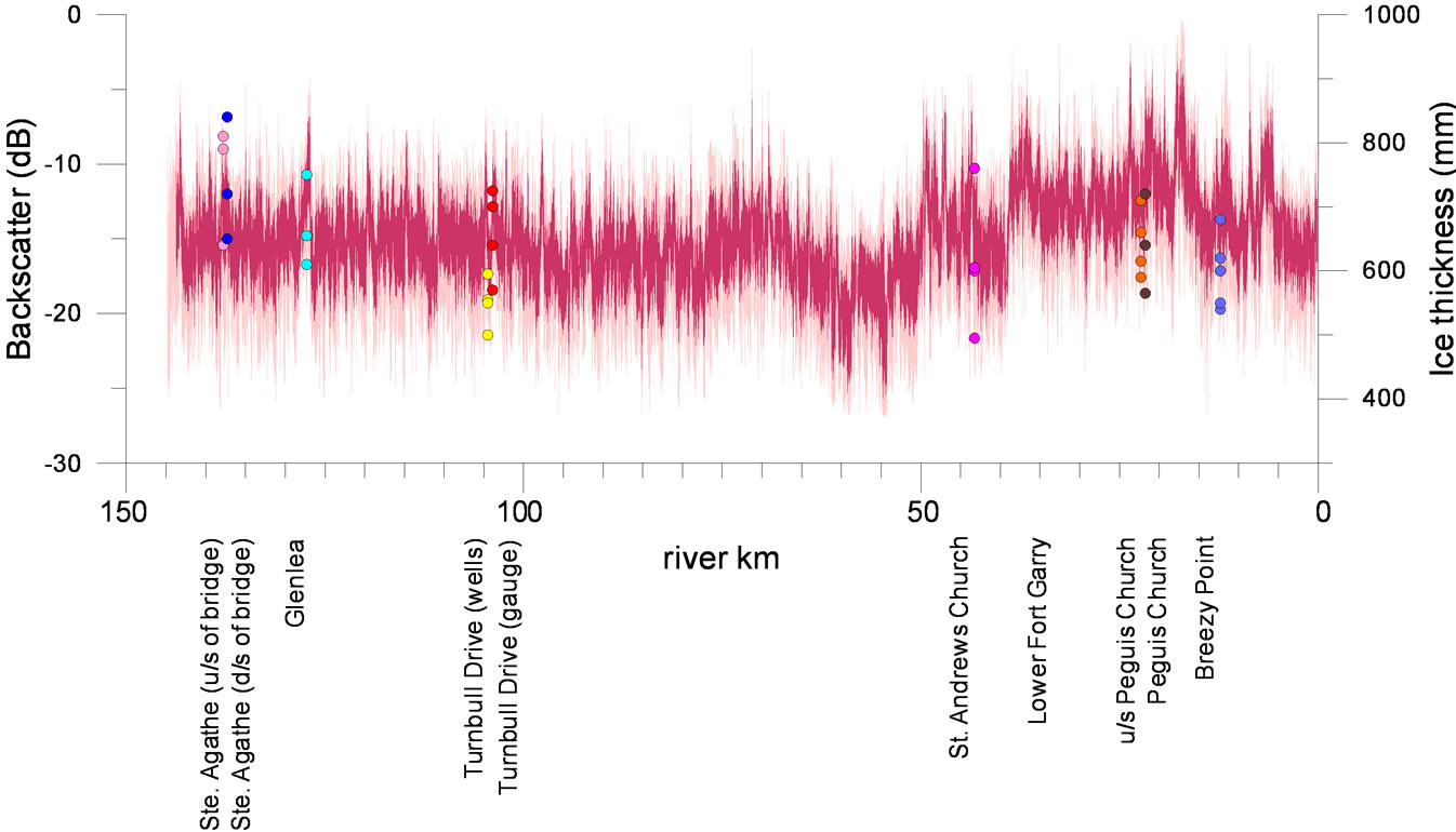
Figure 11. HH backscatter longitudinal profile and ice thickness measurements for March 2010. Dark shading represents the ± 1 standard deviation about the mean; light shading encompasses the maximum and minimum extent of the backscatter values of a moving window along the river centreline. Ice thickness measurements from all drilled holes are superimposed on the graph with dots, each color representing a different transect.
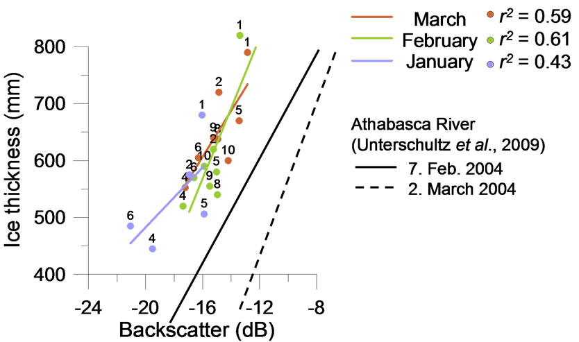
Figure 12. Correlation between mean backscattering and mean ice thicknesses at each transect for the January, February and March surveys in 2010. Results from [11] from the Athabasca River are shown for comparison. Numbers correspond to survey sites in Figure 8.
River (r2 = 0.62 for February and r2 = 0.83 for March). The linear regressions they obtained are superimposed on Figure 12. Their backscatter readings are higher because their images were obtained with the sensor positioned with a lower incident angle (39° - 42°) normal to the earth’s surface. The steeper impingement of the beam onto the ice surface causes more microwaves to be scattered back to the satellite sensor.
The improvement in the backscatter/ice thickness correlation is in line with other studies, primarily of lake ice. Morris et al. [19] observed during the onset of freeze-up that there is a high contrast between undeformed congealed ice (low backscatter return) and ice with deformation features (strong backscatter return). Such features include cracks related to thermal stresses generated as the thin ice cover cools and areas of ridging or rafting which develop as the wind fractures and displaces the initial thin ice (surface scattering). However, as the winter progresses, this contrast in return signal decreases to < 2 dB approximately 8 weeks after freeze-up. The disappearance was attributed to the forward scattering of gas bubbles included in the ice and the increased specular reflection off the basal ice-water interface (volume scattering) [19]. Other lake ice studies ([20,21]) confirm that much of the return signal can be attributed to back scattering from the ice-water interface and some to forward scattering of the bubble inclusions within the ice cover. This suggests that the increase in backscatter during the course of the winter is primarily due to the thickening of the ice.
Another important observation by [19] was that a temporary change in air temperature to > 0℃ may change the nature of the ice and snow cover to cause the contributions of backscatter returned from ice surface deformation features to become much more uniform; differences in the signal return from irregular and smooth surfaces are smoothed out. A warm spell did occur in the watershed during the first week of February 2010 (see Figure 13) during which time such smoothing effects could have occurred so that volume scattering throughout the ice thickness contributed more to the overall signal return than from surface scattering.
In Figure 14, the December ice cover in the mostdownstream reach, whose water levels are impacted by Lake Winnipeg, is overall thinner than in the upstream portion of the study area. However, the ice thickening rate is faster in this reach and the overall ice thicknesses surpass those of the upstream reach by March. Ice thinning is also observed from February to March immediately downstream from the outfalls of wastewater treatment plants (WWTP) and areas of higher flow such as at Lister Rapids.
Snow depth measurements correlated best with HV readings and are superimposed on the HV longitudinal profiles from 10. February 2010 in Figure 15. The best correlation was obtained for the February survey (see
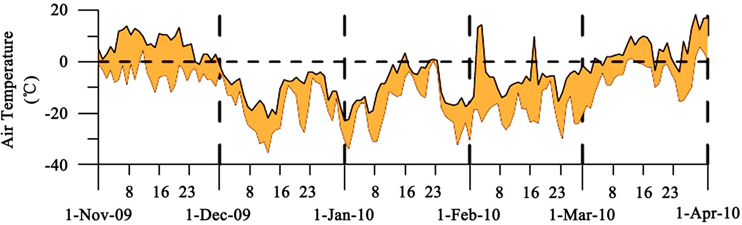
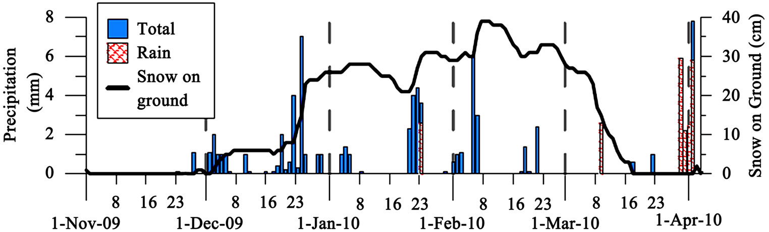
Figure 13. Meteorological data for the winter of 2009–2010. Top panel: Air temperature range between its maximum and minimum daily values at Stony Mountain. Bottom panel: Total precipitation, rain and total snow depth near Oakbank. See Figure 8 for locations of the meteorological stations.
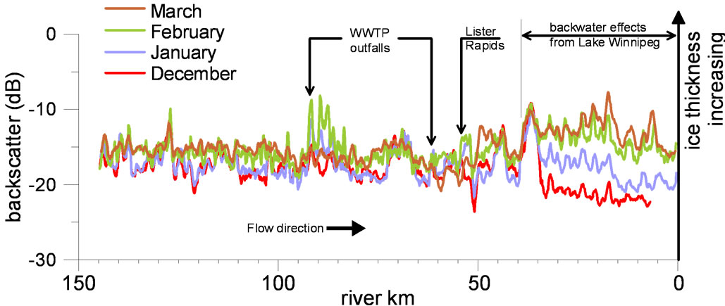
Figure 14. Smoothed longitudinal profile of radar backscatter from Red River ice cover acquired in 2010.
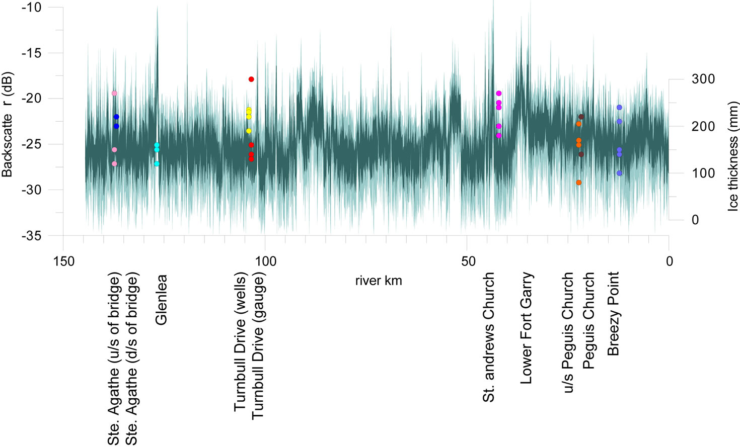
Figure 15. HV backscatter longitudinal profile and snow depth measurements for February 2010. Dark shading represents the ± 1 standard deviation about the mean; light shading encompasses the maximum and minimum extent of the backscatter values of a moving window along the river centreline. Average snow depths near each drilled hole are superimposed on the graph with dots, each color representing a different transect.
Figure 16), after a fresh snowfall of approximately 10 cm on 6. and 7. February 2010 (see Figure 13).
5. Conclusions
Processing imagery from RADARASAT-2 signals is a feasible technique to determine thicknesses of river ice on a large scale. The methodology can be implemented in an operational context during spring flood and ice events along the Red River.
Important observations derived from the study include that HH-backscatter readings correlate better with ice thicknesses averaged at each transect. HV-backscatter readin gs correlate better with depth measurements of fresh snow than with depth measurements of aged snow. Additionally, using same sensor incident angle and flight
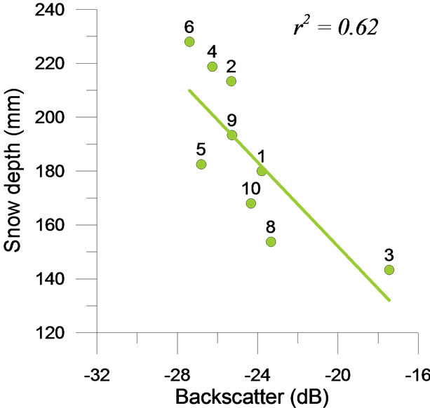
Figure 16. Correlation between mean backscattering and mean snow depths at each transect for the February 2010 survey. Numbers correspond to survey sites in Figure 8.
geometry allows ice thickening rates to be determined.
The large-scale ice thickness readings obtained from the satellite imagery can now be used in an empirical model to determine the probability of ice breakup for different time frames along the Red River. The location and timing of ice breakup is an indication of where ice jams may occur. The breakup forecasting model can then serve as input to a hydrodynamic/ice jam model in order to determine the formation and behaviour of ice jams along the river.
6. Acknowledgements
The authors wish to thank Roy Dixon, an expert in remote sensing techniques, for useful comments on the manuscript while it was being prepared for submission. Many thanks also to the three reviewers for their suggestions which helped strengthen the manuscript.
REFERENCES
- M. P. Lacroix, T. D. Prowse, B. R. Bonsal, C. R. Duguay and P. Ménard, “River Ice Trends in Canada,” Proceedings 13th Workshop on the Hydraulics of Ice Covered Rivers by CGU HS Committee on River Ice Processes and the Environment (CRIPE), Hanover, New Hampshire, 15-16 September 2005.
- B. R. Bonsal and T. D. Prowse, “Trends and Variability in Spring and Autumn 0℃-Isotherm Dates over Canada,” Climatic Change, vol. 57, no. 3, 2003, pp. 341-358.
- S. J. Jones “A Review of the Strength of Iceberg and Other Freshwater Ice and the Effect of Temperature,” Cold Regions Science and Technology, vol. 47, 2007, pp. 256-262.
- E.M. Schulson, “The Structure and Mechanical Behavior of Ice,” Journal of the Minerals, Metals & Materials Society, vol. 51, no. 2, 1999, pp. 21-27.
- B. T. Tracy and S. F. Daly, “River Ice Delineation with RADARSAT SAR,” Proceedings of the 12th Workshop on River Ice, Edmonton, Alberta. 2003.
- F. Weber, D. Nixon and J. Hurley, “Semi-Automated Classification of River Ice Types on the Peace River Using RADARSAT-1 Synthetic Aperture (SAR) imagery,” Canadian Journal of Civil Engineering, vol. 30, no. 1, 2003, pp. 11-27.
- H. Drouin, Y. Gauthier, M. Bernier, M. Jasek, O. Penner and F. Weber, “Quantitative validation of RADARSAT river ice maps,” Proceedings of the 14th Workshop on River Ice, Québec, 2007.
- K.D. Pelletier, J. van der Sanden and F. E. Hicks, “Synthetic aperture radar: current capabilities and limitations for river ice monitoring,” Proceedings of the 17th Canadian Hydrotechnical Conference, Edmonton, Alberta, 17-19 August 2005, pp. 1-10.
- Y. Gauthier, F. Weber, S. Savary, M. Jasek, L. M. Paquet and M. Beriner, “A Combined Classification Scheme to Characterise River Ice from SAR Data,” EARSel eProceedings, vol. 5, No. 1, 2006, pp. 77-88.
- M. Jasek, F. Weber and J. Hurley, “Ice Thickness and Roughness Analysis on the Peace River using RADARSAT-1 SAR Imagery,” Proceedings of the 12th Workshop on River Ice, Canadian Geophysical Union—Hydrology Section, Communication on River Ice Processes and the Environment, Edmonton, Alberta, 18-20 June 2003, pp. 50-68.
- K. D. Unterschultz, J. van der Sanden and F. E. Hicks, “Potential of RADARSAT-1 for the Monitoring of River Ice,” Cold Regions Science and Technology, vol. 55, 2009, pp. 238-248.
- J. J. van der Sanden, H. Drouin, F. E. Hicks and S. Beltaos, “Potential of RARARSAT-2 for the Monitoring of River Freeze-Up Processes,” Proceedings of the 15th Workshop on River Ice, CGU HS Committee on River Ice Processes and the Environment, St. John’s, Newfoundland and Labrador, 15-17 June 2009, pp. 364-377.
- CCRS, “Fundamentals of Remote Sensing,” Canada Centre for Remote Sensing, 2009.
- M. Hallikainen and D. P. Winebrenner “The Physical Basis for Sea Ice Remote Sensing,” In: F. Carsey, Ed., Microwave Remote Sensing of Sea Ice, American Geophysical Union Geophysical Monograph, Washington, D.C., 1992, pp. 29-46.
- S. Sandven and O. M. Johannesen “Sea Ice Monitoring by Remote Sensing,” In: J. F. R. Gower, Ed., Manual of Remote Sensing: Remote Sensing of the Marine Environment, 3rd Edition, Vol. 6, American Society for Photogrammetry Remote Sensing, Bethesda, 2006, pp. 241- 283.
- D. G. Barber, D. G. Flett, R. A. de Abreu and E. F. LeDrew, “Spatial and Temporal Variation of Sea Ice Geophysical Properties and Microwave Remote Sensing Observations: The SIMS’90 Experiment,” Arctic, vol. 45, no. 3, 1992, pp. 233-251.
- M. Mäkynen, “Investigation of the Microwave Signatures of the Baltic Sea Ice,” Dissertation at Helsinki University of Technology, Espoo, Finland, 2007.
- MDA, “RADARSAT-2 product description,” MacDonald, Dettwiler and Associates Ltd., 2009.
- K. Morris, M. O. Jeffries and W. F. Weeks, “Ice Processes and Growth History on Arctic and Sub-Arctic Lakes Using ERS-1 SAR Data,” Polar Record, vol. 31, no. 177, 1994, pp. 115-128.
- M. O. Jeffries, K. Morris and W. F. Weeks, “Structural and Stratigraphic Features and ERS-1 Synthetic Aperture Radar Backscatter Characteristics of Ice Growing on Shallow Lakes in NW Alaska, Winter 1991-1992,” Journal of Geophysical Research, vol. 99, no. C11, 1994, pp. 22459-22471.
- C. R. Duguay, T. J. Pultz, P. M. Lafleur and D. Drai, “RADARSAT Backscatter Characteristics of Ice Growing on Shallow Sub-Arctic Lakes, Churchill, Manitoba, Canada,” Hydrological Processes, vol. 16, No. 8, 2002, pp. 1631-1644.