Journal of Water Resource and Protection
Vol. 1 No. 2 (2009) , Article ID: 609 , 19 pages DOI:10.4236/jwarp.2009.12010
Long-Term Study of Lake Evaporation and Evaluation of Seven Estimation Methods: Results from Dickie Lake, South-Central Ontario, Canada
Dorset Environmental Science Centre, Ontario Ministry of Environment, Dorset, Ontario, P0A 1E0, Canada
E-mail: huaxia.yao@ontario.ca
Received March 31, 2009; revised April 20, 2009; accepted May 4, 2009
Keywords: Long-Term Study, Lake Evaporation, Water Balance, Energy Budget, Lake Temperature, Stream Discharge
ABSTRACT
Establishing satisfactory calculation methods of lake evaporation has been crucial for research and management of water resources and ecosystems. A 30 year dataset from Dickie Lake, south-central Ontario, Canada added to the limited long-term studies on lake evaporation. Evaporation during ice-free season was calculated separately using seven evaporation methods, based on field meteorology, hydrology and lake water temperature data. Actual evaporation determined during a portion of a year was estimated using a lake energy budget model, and the estimation was used as reference evaporation for evaluation of the seven methods. The deviation of method-induced evaporation from the reference evaporation was compared among the seven methods, and a performance rank was proposed based on the root mean squared deviation and coefficient of efficiency. As for the whole ice-free season (roughly May to November), the water balance was the best method, followed by Makkink, DeBruin-Kejiman, Penman, Priestley-Taylor, Hamon, and Jensen-Haise methods. As for shorter duration (a week to a month), the DeBruin-Kejiman was the best method, followed by Penman, Priestley-Taylor, Makkink, Hamon, Jensen-Haise, and water balance method. Annual and seasonal changes of energy budget terms and the compensation function of lake heat storage in evaporation flux were also analyzed.
1. Introduction
Natural lakes and artificial reservoirs provide a valuable water resource. The quantity and quality of lake water resource are important for agriculture, fisheries, recreation, domestic and industrial water supply, aquatic ecosystem, and hydropower [1-2]. Lake water availability is regulated by the water balance and energy budget processes which in turn are closely tied to climate variations, land use change or other human influences [3-5]. For example, a common indicator of water availability – lake water level – is influenced by four major processes or factors: 1) precipitation on the lake and its drainage watersheds; 2) surface and subsurface runoff generated from the watersheds; 3) runoff leaving the lake; and 4) direct evaporation loss from the lake surface. Therefore, it is crucial to understand the lake evaporation process, establish satisfactory calculation methods, and identify the effects of lake evaporation on lake level and water resources.
Long-term observations and field data are important for understanding lake evaporation, creating estimation methods, and evaluating effects of evaporation change (caused by climate change or land use change) on water resources. However, it is challenging or difficult to directly measure lake evaporation for a long time, because it involves significant financial investment in instruments, field maintenance, and field work on a lake. Usually lake evaporation is estimated or calculated by a formula and using regular meteorological and hydrological data. Lake evaporation is affected not only by climatic variables, but also by lake characteristics such as depth, surface area, and water clarity and temperature. Lake water itself influences the energy budget and lake evaporation through the changes in water temperature and water mixing (turn over). Accurate accounting of energy budget processes requires observations of temperature profiles of lake water. As a result, these field difficulties have severely restricted the number of long-term evaporation studies.
Methods, equations or models for determining lake evaporation may be categorized into four categories: energy budget, aerodynamic transfer (or mass transfer), combination of aerodynamic transfer and energy budget, and empirical method. Most literature studies using one or more of these methods have utilized short-term field monitoring and datasets. In this paper “long-term” studies mean those that conduct and utilize monitoring data of multiple years to more than 5 years. Lenters et al. [6] completed a comprehensive study of lake evaporation and effects of climate variation by using 10 year data from a small lake in Wisconsin USA. In the article by Lenters et al., some long-term studies were summarized. Apart from these summarized examples, there are other long-term studies that have been conducted: a lake in Northwest Territories of Canada for six years [7], the small Lake Kinneret in Israel for five years [8], the large Lake Okeechobee (1732 km2) in Florida USA for five years [9], a small reservoir (8.8 km2) in Minas Gerais State, Brazil for three years [10], the large man-made Lake Mead (506 km2) in Las Vegas, Nevada USA for three years [11], the large Bear Lake in Idaho and Utah, USA for two years [12], the Cottonwood Lake Area in North Dakota USA for 5 years [13], the Mirror Lake in New Hampshire USA for 6 years [14], the Perch Lake in eastern Ontario Canada for 11 years [15], several lakes in Minnesota USA for 11 years [16], and several more examples using two-year data [17-19]. Scheider et al. [20-21] and Hutchinson et al. [22] have reported on lake evaporation study of 15 years (1976–1992) for lakes in Muskoka area of Ontario, Canada.
The study examples mentioned above are listed in Table 1, illustrating the limited number of long-term studies. There are only 14 examples of studies in Table 1 where five or more years of data are used. The Lake Ziway study with the longest data record of 30 years made many simplifications in its calculations of monthly and annual average evaporation and did not provide details of the evaporation process. Therefore, additional studies of lake evaporation using long-term data are needed to describe the evaporation process and its variability; and to confirm and compare the applicability of available estimation methods. A detailed analysis of 30 year (1978–2007) field data for Dickie Lake (the lake is located in the same Muskoka-Haliburton area as monitored and reported by Scheider et al. and Hutchinson et al.) is presented in this paper.
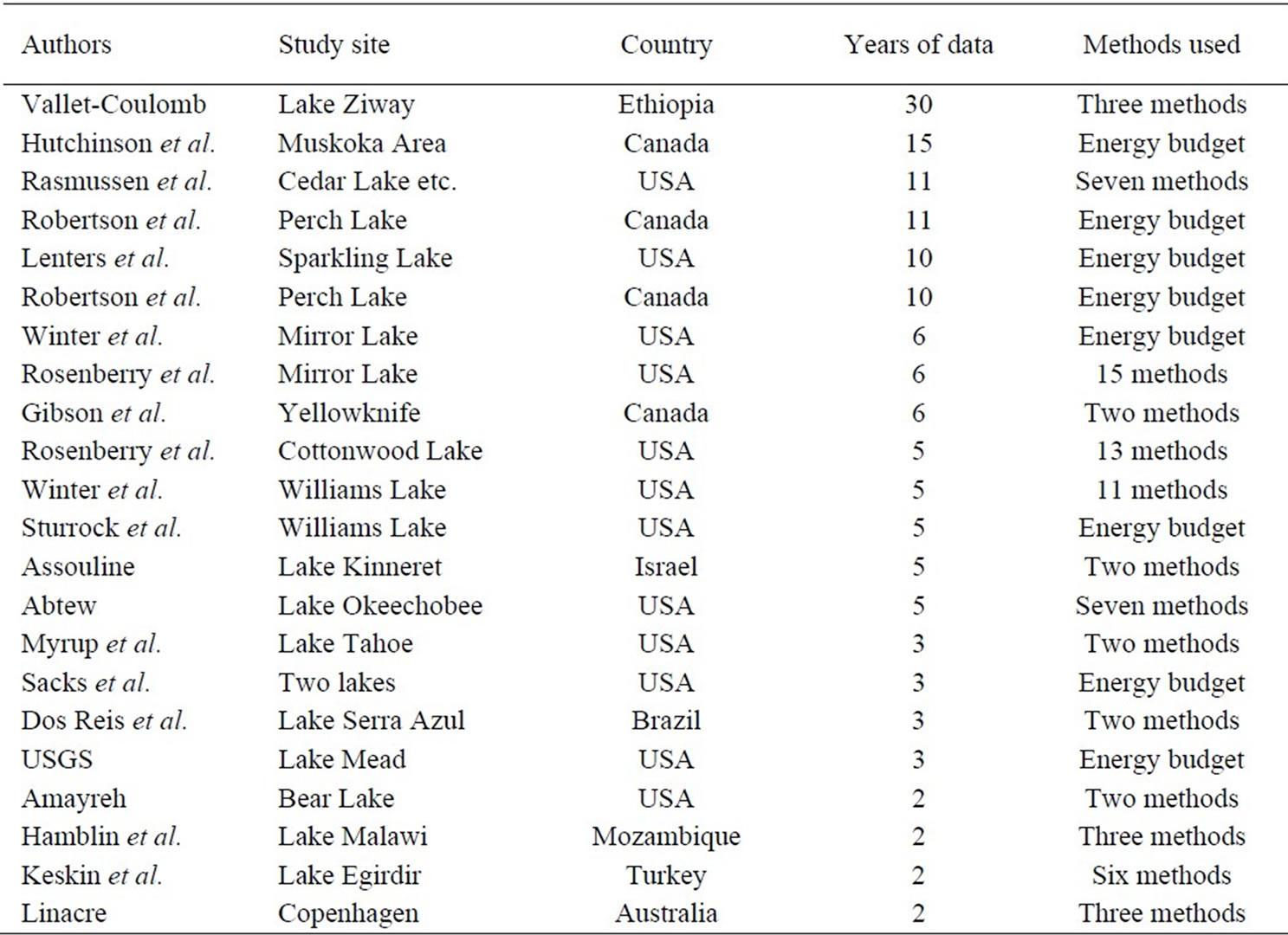
Table 1. Study examples of long-term lake evaporation.
Apart from the need for long-term data, methods for evaporation estimation should be discussed and assessed, because more than 30 methods or equations have been proposed and most of them perform differently for different geographical areas. Winter et al. [23] compared 11 well-used methods with the energy budget method by using high-quality data for five years from Williams Lake, and proposed a ranking based on best to least performance. Their ranking is: Penman, DeBruin-Kejiman, Makkink, Priestley-Taylor, Hamon, Jensen-Haise, mass transfer, DeBruin, Papadakis, Stephens-Stewart, and Brutsaert-Stricker. Rosenberry et al. [13,14] compared as more as 15 methods with energy-budget method using 6-year data and proposed their ranking. Rasmussen et al. [16] compared seven methods for use in lake temperature modeling. The evaluation of seven methods by Abtew [9] suggested that simple models (such as the modified Turc model only using solar radiation and maximum air temperature) could perform better than Penman-combination or Priestley-Taylor model requiring many more parameters. The four methods–Priestley-Taylor, DeBruin-Kejiman, Papadakis and Penman were compared with energy budget by Mosner and Aulenbach [24] using single-year data, and the Priestley-Taylor was found to be the best of the four methods. Xu and Singh [25] tested eight radiation-based evaporation models in order to estimate future lake levels. Singh and Xu [26] evaluated 13 mass-transfer equations against pan evaporation data. Delclaux et al. [27] compared five monthly evaporation methods and the best results of lake evaporation were obtained by the Abtew model and Makkink model. Comparisons of estimation methods were also made by Keskin and Terzi [18] and Sadek et al. [28]. All these comparisons provided somehow different conclusions depending on sites and data used.
As indicated by Winter et al. [23], earlier comparisons of evaporation methods did not use extensive or long term data. Also comparisons have been focused more on large lakes in arid and semiarid climates than on small lakes in humid and sub-humid climates. The lakes in cold or boreal ecozones (such as those located on the Canadian Shield) have received even less attention. The evaluation of methods needs to be made for a longer period of time, a wider scope of lake sizes and more climatic settings. In our study, seven commonly used methods are compared with each other and assessed by using long-term data from Dickie Lake on the Canadian Shield where such comparison has rarely been made. Only one case of method comparison was reported for Canadian Shield: Singh and Xu [26].
Another issue in evaporation studies is the standard or reference that was used to verify estimation methods. Actual lake evaporation can be measured by an instrument such as the eddy covariance system, but long-term data from the system has not been reported. A common measure of lake evaporation is by using an evaporation pan, with a limitation: the pan coefficient (multiplying the coefficient with the pan evaporation data to get lake evaporation) depends on season, location and the specific pan in use [9]. In case a reliable and direct measure of long-term evaporation did not exist, many reported comparison studies chose to evaluate methods by comparing evaporation results with that of an energy budget method, as the latter was considered the best method to estimate lake evaporation [6,13,14,23,24]. In our study of Dickie Lake, there was no data from pan evaporation or eddy covariance instrument, the energy-budget results were used to be the reference for evaluating performance of other estimation methods.
Therefore, our study has three goals: 1) provide an evaporation study using long-term 30-year datasets obtained for a small lake located in the Canadian Shield region; 2) estimate evaporation of ice-free season for 30 years using seven methods, and discuss their applicability to cold ecoregions; and 3) compare deviations of method-calculated evaporation to the energy-budget-estimated evaporation, and identify the better methods for estimating lake evaporation for the region.
2. Site and Data Description
The Muskoka-Haliburton study region as shown in Figure 1 is located in south-central Ontario, Canada, to the east of Lake Huron, one of the five Great Lakes in North America. Environmental monitoring programs including hydrological and meteorological observations were started and managed by the Dorset Environmental Science Centre, Ontario Ministry of the Environment in 1976, and have been continuous till present. The program includes nine lakes and their contributing watersheds, as representatives of inland lakes on the Canadian Shield landscape, which typically consists of exposed bedrock and numerous lakes. The lakes and watersheds in the MuskokaHaliburton study area drain into Muskoka River or Gull River which contributes to Muskoka Lake and finally into Georgian Bay of Lake Huron. The region is relatively undeveloped by humans, with the exception of small towns or villages like Huntsville, Bracebridge or Dorset, and some scattered cottages alongside shorelines or in forested areas.
The study lake, Dickie Lake, is one of the nine lakes (Figure 1, Number 6), and is located between Bracebridge and Dorset, about 20 km from both. The lake, streams and drainage watersheds, and monitoring gages are shown in Figure 2. There are five main streams going into the lake, and their watersheds are numbered as 5, 6, 8, 10 and 11 in Figure 2. These stream watersheds occupy a large portion of the total drainage area. There is a weir (gauge) at the end of each stream to monitor water levels at that particular point and the levels are converted to stream discharges with calibrated level-discharge relationships. A small portion of the drainage area, which is close to the lake’s shoreline and does not have obvious streams, has not been monitored by gauges. The outflow on the south-west side of the lake is also monitored. The lake’s water level is observed at a location off the inlet of watershed 6. The areas of the five main watersheds are 0.30, 0.22, 0.67, 0.79, and 0.76 km2 respectively, giving a gauged drainage area of 2.74 km2. The ungauged drainage area is 1.32 km2 whereas the total drainage area is 4.06 km2. The lake itself has an area of 0.94 km2. The lake’s outlet point controls a total area of 5.0 km2.
The geology of Dickie Lake drainage area is composed of three surficial geology types [21]: shallow surficial deposits (less than 1 m in depth) covering 78 % of the area, deep surficial deposits (greater than 1 m in depth) covering 3 %, and organic soils covering 19 %. Therefore, the soil is thin and poorly developed, making surface runoff the dominant runoff generation while groundwater runoff from bedrock is minimal. Forest cover is almost continuous in the watershed although it contains some areas of exposed bedrock. The percentages of wooded land and exposed bedrock among the whole watershed are 83 % and 17 % respectively. Small logging operations and dwellings around the lake and watershed exist, but their influence on the hydrological cycle is minimal. Consumptive use of lake and stream water is also minimal.
The climate of the study area is cold and humid in fall and winter, with less precipitation in summer than in fall or winter, and usually has significant snow/ice melting in spring. As presented by the data records, annual mean air temperature is 4.9 °C, and average annual precipitation is 1010 mm.
The data collection and processing was completed using a meteorology station located at Heney Lake approximately 1.0 km away from Dickie Lake (Figure 1). The data used for calculations include daily precipitation, daily mean temperature, relative humidity, wind speed, and daily global radiation. This station provides a majority of data used for the Dickie Lake study. When a data point was missing or unreliable at the Heney station, three other nearby stations located close to Chub Lake, Plastic Lake and Harp Lake were used to give a proper data value. The processed data are available for 30 years: 1978–2007.

Figure 1. Locations of study area and study lake.

Figure 2. Dickie Lake and its watersheds (W and F mean stream gauge type: weir and flume).
Stream water level data are obtained from field recording charts which are used to provide hourly and daily discharges for five watershed streams. Daily mean discharges are available for 30 years: 1978–2007. They are used for evaporation estimation via lake water balance calculations.
Lake temperature profiles (water temperature at 1 m intervals from lake surface to lake bottom) were conducted at one and central point of the lake, on varying dates throughout a year, mostly during the ice-free season. A period between two observation dates consists of 6 to 45 days, two weeks on average. The water depth measured at the deepest and central part of the lake varies between 9 and 12 meters, therefore, the number of vertical profile zones changes slightly in the year, with one zone being one meter thick. Available data covers a period of 30 years (1978–2007).
Lake levels were monitored once every two or three weeks on average, during ice-free season only, for 23 years: 1980 to 2002. They are used to calculate water balance.
For clarification, the three timing concepts used in the study are explained. Lake temperature profile observation begins in early May but not fix on a specific date, ends in mid November. The time length between any two observation dates is called a “period”. A period has a range of 6 – 45 days depending on actual field work, and is used for evaporation calculations. The lake level observation begins in May and ends in November (differs between years, and differs from the lake profile observation dates). The time length between two observation dates is called an “interval”. A period and an interval may cover some same days, but do not necessarily coincide completely with each other, as water temperature and lake level may not be observed on a same date. An interval has a range of 2 – 34 days, and is used for water balance calculations. The length of whole ice-free time appointed in the study, or the total cumulative time over all intervals in a year, is called a “span”. It starts from the earliest day of lake level observations that falls within the periods and ends at the last day of level observations falling into the periods. The span for water balance is 68 – 190 days long depending on the year.
The concept “period” is important for calculating the evaporation using any lake-heat-storage-based method, because only the first day and last day of the period have observations of the lake’s temperature profile which is needed to know lake heat storage. For those methods using lake temperature data, total evaporations in periods have to be calculated before a daily evaporation rate averaged over the period can be known or the daily rates are approximately allocated (see a later allocation explanation). For other methods not using lake temperature data, daily evaporation can be calculated first, and the periods are not necessarily required. However, for consistency, the periods are used for all methods in this study.
Listed in Table 2 is the number of periods of each year, number of consecutive days covered by the periods, number of intervals, and span length in a year. For example, there are 21 periods in 1980 which cover 180 consecutive days (from Julian day 126 to 305), and 17 intervals which cover 141 days (the span from Julian day 162 to 302). There are no intervals assigned for years 1978 and 1979 as the lake level monitoring was started in 1980, and no intervals for years 2003–2007 as recorded level data in these years were found unreliable.
3. Methods
3.1. Reference Evaporation Derived by Energy Budget
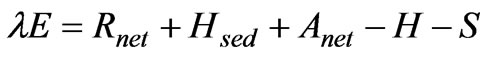
The energy budget is often used for lake evaporation calculations. For a lake and for a given time period previously defined, its energy budget is written as
 (1)
(1)
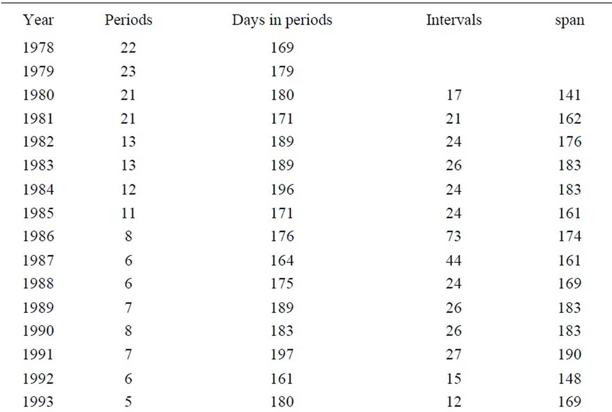

Table 2. Calculation periods and intervals.
where all energy terms are in unit of Joule. λE is latent energy used by evaporation of lake water during the period, λ is the latent heat of vaporization (2.46×10⁶ J kg-1), E is the evaporation (mm) within the period, Rnet is net radiation, Hsed is heat released by lake sediments and is negligible for most cases, Anet is net heat advected into the lake from precipitation, inflows and outflows, and is also negligible, H is sensible heat transfer from lake surface to atmosphere, and S is the change of heat stored in the lake (due to temperature changes) during the period. The negligibility of the net heat advection Anet could be supported by the study results of Lenters et al. [6] for Sparkling Lake (0.64 km2, similarly small as Dickie Lake’s area 0.94 km2). They found that this advection term only had a mean value of 0.1 W m-2 in 10 summers, very small compared to other energy budget components (107 W m-2 of Rnet, or 89 W m-2 of λE). Although a lacking of stream water temperature data at our site does not warrant a rigorous calculation of the advection term, it is believed negligible.
The sensible heat term can be expressed as H=B· λ E, where B is the mean Bowen ratio for the period. Removing the two negligible terms, Equation (1) is rewritten as
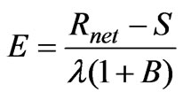 (2)
(2)
The net radiation is an accumulation of daily net radiation in the period:
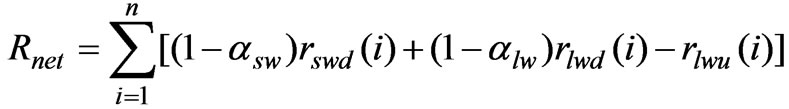 (3)
(3) where i is the order of any day in the period (i=1, 2, ……, n days), rswd(i) is daily downward shortwave radiation which is observed at the meteorological station, αsw=0.07 is the shortwave albedo of water (value taken from Lenters et al. [6]), rlwd(i) is daily downward longwave radiation, αlw=0.03 is the longwave albedo, and rlwu(i) is daily upward longwave radiation. Longwave radiations are calculated by rlwd(i)=εaσTa4, rlwu(i)=εsσTs4, where εa=0.91 and εs=0.97 are emissivity of the atmosphere and surface water respectively, Ta and Ts are daily air temperature and surface water temperature (in unit of ˚K). The daily air temperature is provided by routine monitoring, while surface water temperature is observed only on the first and last day of a period (roughly 14–21 days long). The daily water temperature within a period is obtained by interpolation between the two days’ temperature values.
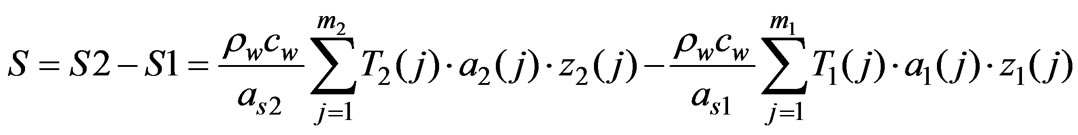
The heat storage change S in Equation (2) is calculated by using vertical lake zones and lake temperature profiles. Temperature profiles are observed at the central lake where it has the deepest water. The water body is divided into vertical zones from lake surface to lake bottom, and the number of zones may differ a little among periods. The heat stored in the lake on the last and first day of the period is calculated, and their difference is the change in heat storage,
 (4)
(4)
where S2 and S1 are heat storage on the last and first day respectively, ρw=1000 kg m-3 is water density, cw=4186 J kg-1 ˚C-1 is specific heat of water, as2 and a2(j) are the lake surface area and water area (m2) of any zone j (j=1, 2, ……, m2 starting from the lake surface zone) on the last day, T2(j) and z2(j) are the temperature and thickness of zone j on the last day. Similarly, as1, a1(j), T1(j), z1(j) are the surface area, water area, water temperature and zone thickness respectively on the first day. Water area a (m2) at a height h (m) from lake bottom is estimated by an empirical relation derived from observed lake morphometry data [29] as follows.
 (5)
(5)
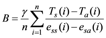
As in Equation (6), the period-mean Bowen ratio B is calculated from daily Bowen ratios which is derived from air and lake surface temperatures [30].
 (6)
(6)
where γ is psychrometric constant (67 Pa ˚C-1), n is the number of days in a period, i is any day within a period, Ts(i) and Ta(i) are daily mean temperature (˚C) of lake surface and air above the lake respectively, ess(i) and esa(i) are saturated vapour pressure (Pa) at the lake surface and air temperatures. The saturated vapour pressure is calculated with the Arden Buck Formula [31]:
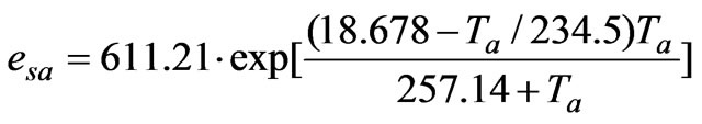 (7)
(7)
Daily evaporation is not obtained by using Equation (2) as the field collection of lake temperature profiles is not conducted every day in a period. After the total evaporation E is calculated as above, daily evaporation is allocated from the total amount based on a distribution pattern. Hamon method is the easiest way to estimate daily evaporation and uses only air temperature. Therefore, a time series of daily evaporation is created by using the Hamon method (described later), their summation gives a total amount, and the ratio of daily evaporation to total evaporation is determined. By applying the same ratios to the total amount value obtained from the energy budget method, daily evaporations for the energy budget method are obtained. A further discussion on the allocation caveat will be provided in the Discussion section.
3.2. Evaporation Methods
Seven methods are selected for calculation of lake evaporation at Dickie Lake and are later compared to each other. They are Hamon (HM), Penman (PM), Priestley-Taylor (PT), DeBruin-Kejiman (DK), Jensen-Haise (JH), Makkink (MK) and water balance (WB). These methods are commonly used and once compared in literature, but they have not been compared or evaluated for lakes on the cold Canadian Shield, using dataset as long as 30 years. Water balance method has not been compared with other methods in the published reports. Calculations are conducted for the defined periods of each year, and two values are estimated – the total evaporation amount in a period, and daily evaporation rates for the period. Depending on individual methods, the total evaporation is given first, then daily rates are calculated from the total value; or the daily evaporation rate is calculated first, then the total value is derived from daily rates. Comparisons of the seven methods are made on basis of interval and span, not on daily basis. However, daily evaporation rate is required to provide the evaporation amount within an interval, as the dates in an interval are different from the dates in a period.
3.2.1. Hamon Method
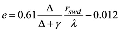
It is often used to estimate lake evaporation or watershed potential evaporation because of its simplicity [32]. For a given lake, daily evaporation e (mm) is calculated from daily temperature Ta (˚C) as follows.
 (8)
(8)
where D is the ratio of maximum sunshine duration (hour) to 12 hours, and is determined by latitude of the lake and the date:
 (9)
(9)
where φ is the latitude (45.13˚ for Dickie Lake), J is the Julian day of any date of interest.
Total evaporation E in a period is the sum of daily evaporations of all included days.
3.2.2. Penman Method
A format of Penman equation, once recommended by Food and Agriculture Organization [33], is used and slightly modified to calculate lake evaporation. The modification is an addition of the lake heat storage change rather than taking only the net radiation. The evaporation in a period is written as
 (10)
(10)
where Rnet and S are the net radiation (Joule) and lake heat storage change in the period,  is the mean daily wind speed (m s-1) for the period,
  is the mean daily relative humidity (≤1.0),
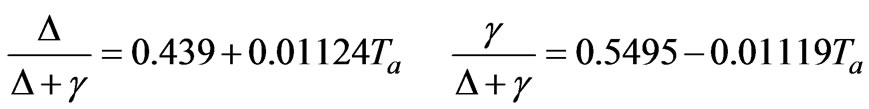
  is the mean daily saturated vapour pressure (Pa), Δ is the mean slope of the saturated vapour pressure – temperature curve at the air temperature, and n is number of days in the period. The two terms related to the slope Δ and psychrometric constant γ are expressed as empirical relations of air temperature [34]:
 (11)
(11) Total evaporation is obtained first as the lake heat storage change in a period (S) is included in Equation (10). The total evaporation E is allocated to each day of the period as done for the case of energy budget.
3.2.3. Priestley-Taylor Method
Evaporation is estimated based on radiation and heat storage only, as done by Winter et al. [23].
 (12)
(12)
where the variable Δ/(Δ+ γ) is estimated in Equation (11).
3.2.4. DeBruin-Kejiman Method
The DeBruin-Kejiman equation is written as [23,35]
 (13)
(13)
where the slope of saturated vapour pressure curve Δ could be estimated by using Equation (11), and net radiation and lake heat storage change have been estimated in the energy budget calculations.
3.2.5. Jensen-Haise Method
Daily evaporation is first calculated by the following Equation [23].
 (14)
(14)
where Ta is daily temperature (°C), rswd is daily shortwave radiation as used in Equation (3). The total evaporation in a period is the sum of the daily rates.
3.2.6. Makkink Method
Daily evaporation is calculated as [23]
 (15)
(15)
And then the total evaporation is obtained.
3.2.7. Water Balance Method
As shown in Figure 2, the lake’s inflows from five major streams are measured, the inflows from ungauged watersheds can be prorated from measured flows, and the lake outflow, lake level and precipitation are also known. Therefore, the lake evaporation during a time span (or interval) can be estimated by using a water balance equation for the lake.
Water balance analysis is made for a time in ice-free season (early May – mid November) as long as the lake level data are available. For a span in a year, the water balance is expressed as
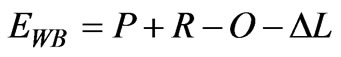 (16)
(16)
where EWB is the total evaporation (mm) during the span, P is the precipitation volume (mm) during the span, R is the runoff (mm) from all watersheds (gauged and ungauged), O is the outflow volume at the lake outlet, and ΔL is the level change over the span.
The span length of a year varies with years, because the starting date and ending date may differ between years. Water balance estimation must begin and end at a day when the lake level is known. After an estimation is completed for a year (May to November usually), a new estimation for the next year is made. Regarding the inflow from ungauged watershed area, a proration method was applied to the study area [20,22] to derive discharge from ungauged area based on the assumption: the areal runoff is equal among the lake’s watersheds. An evaluation of errors originated by the proration was made by Devito and Dillon [36] using two lakes other than Dickie Lake in the same region, and the errors were within 10% of the annual runoff measured. Therefore, we use the same method to get an estimation of the ungauged runoff.
Groundwater inflow and outflow, or groundwater net flow to the lake, are not included in Equation (16) as they are assumed negligible. This assumption was applied to the study area before [20,22,36], and was used in other regions [37]. The characteristic shallow surficial till and largely impermeable bedrock in the Canadian Shield region support the assumption, as it is supported by the small ratio 0.07 of groundwater inflow against surface water inflow to Lake Michigan [38], and by a satisfactory analysis of water balance in 30 years for Dickie Lake without including groundwater flow [Yao et al., Data Report in editing, Ontario Ministry of Environment].
A similar equation as Equation (16) is applied to any interval within a span, and the evaporation amount of the interval is obtained.
3.3. Comparison and Evaluation of Seven Methods
The difference of method-calculated evaporations from the energy-budget EWB values is used as an accuracy index of an evaporation method. Comparing the differences of seven methods will provide a quantitative evaluation of their performance and accuracy. The root mean square deviation (RMSD) is a frequently-used measure of the differences between values predicted by an estimator and the values observed from the thing being estimated. Another indication of how well the estimator follows/predicts the variations in the measured values could be given by a coefficient of efficiency (CE) as proposed and applied by Nash and Sutcliffe [39]. This CE index is expressed as
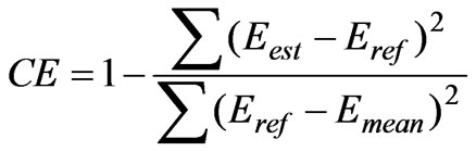 (17)
(17)
where Eest and Eref are the estimated and reference (or measured) evaporation for a span (or interval) respectively, and Emean is the mean of reference evaporations. A larger CE number indicates a more accurate estimator.
Both indexes RMSD and CE are used in our study to evaluate and compare the accuracy and performance of the seven evaporation methods, and a performance rank is then proposed. The estimated evaporation is plotted against the reference evaporation for examining each method’s bias and errors. The comparison is conducted separately for the span (longer time) and interval (shorter time) because a method might perform quite differently between the two time scales.
4. Results
Results of energy budget calculation for 30 years (1978–2007) and the resulted reference evaporation used for comparison are presented first. They are followed by the results of evaporation estimated with the seven methods. Then method comparison results are presented.
4.1. Energy Budget
Span-mean values of energy budget variables (net radiation, sensible heat flux, evaporative heat flux, and lake heat storage rate) and meteorological variables are illustrated in Figure 3 to show their inter-annual changes. Figure 3(a) shows the meteorological variables, and Figure 3(b) shows the energy budget fluxes, with the source
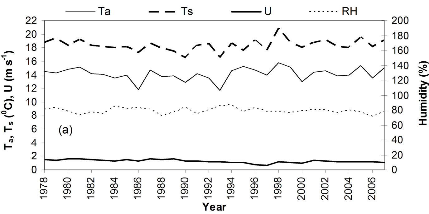
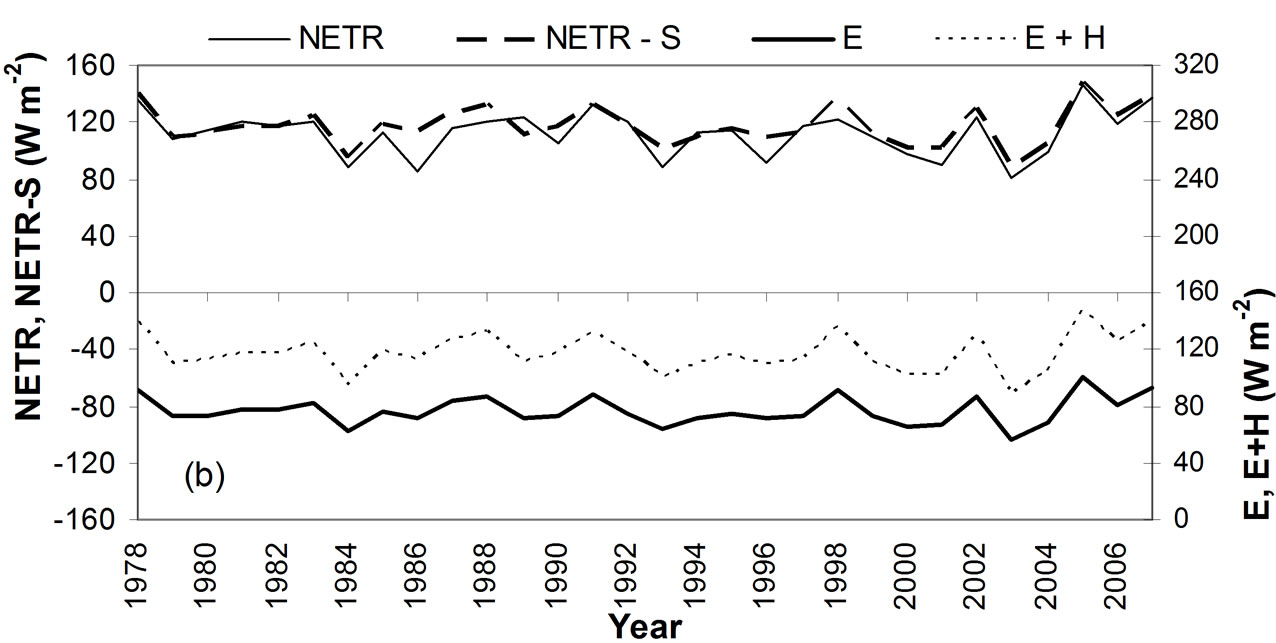
Figure 3. Span averages of (a) meteorological variables, and (b) energy budget variables.
items in upper section and consumptive items in lower section. Air temperature and lake surface temperature change in an identical way, as is usually expected. Net radiation flux changes coincidently with temperature. Very little correspondence is seen between humidity (or wind speed) and temperature (or net radiation). Furthermore, lake heat storage rate possesses a tiny portion in source energy (net radiation - heat storage). For a majority of 30 years, the lake heat storage contributes very little to the energy source on annual basis. For this reason, the consumptive term (E or E+H) has a strong correspondence to net radiation flux: climbing or dropping in the same years.
Daily mean values of meteorological and energy budget variables (the 30-year mean for any day between the Julian day 121 and 319) are illustrated in Figure 4 to show seasonal changes. Air temperature has some fluctuations while demonstrating a clear curving. Corresponding to air temperature, the lake surface temperature has a similar changing curve, but smoother. To their contrast, relative humidity does not have clear seasonal change although it increases slightly, nor does wind speed have clear changes.
The seasonal patterns of energy terms demonstrate two phenomena. 1) The energy source (net radiation minus lake heat storage change, NETR - S) determines how much energy could be consumed by sensible and evaporative fluxes, therefore the source term NETR-S and consumptive term E+H have the same changing pattern – climbing in the summer to their peaks in mid July (around day 200) and dropping in the late summer and fall. 2) There is a time lag between net radiation NETR and consumption E+H, because of the function of lake heat storage. Unlike E+H, net radiation is high in May and June, and then decreases quickly in July and August till November. By dividing the curves at the Julian day 200 (July 20), lake water uses net radiation to increase its temperature or increase heat storage over the first section of the curve, the usable energy source for evaporation and sensible heat conduction is less than the net radiation, and therefore, the high radiation rate does not produce a high E+H rate in May and June. In July the lake is not absorbing net radiation and the high radiation finally creates the highest evaporation rate. Contrarily, lake water reduces its temperature over the second section of the curve, and releases its stored heat to compensate for the decreasing radiation. The usable energy source is more than the net radiation. E+H does not decrease as quickly as the net radiation because of the lake heat compensation. Especially in late October and November, energy provided by lake water overrides the net radiation to maintain a small evaporation flux.
The total reference evaporation in a span of a year, as calculated with the energy budget equations, fluctuates irregularly because of its natural changes with meteorological inputs and the difference in span length (number of days in a span differs, see Table 2). The reference evaporation in a period among the 30 years (totally 326 periods) has large fluctuations too, because a period can be in the hot summer or cold fall, and the period length can be quite different. Therefore, these total reference evaporations are not plotted in a figure. But they will be the basis for methods comparison. In order to illustrate the inter-annual variations in evaporation rates, all daily evaporation rates within a span of a year (121–198 days depending on the year, see Table 2) is averaged to obtain the annual average rate, and the average rates over 30 years are shown in Figure 5. The rate varies between 2.0 – 3.5 mm/d, with lower rates in 1979–1986 and 1999–2004, and higher rates in 1987–1992 and 2005–2007. Not a clear increase or decrease trend is found.
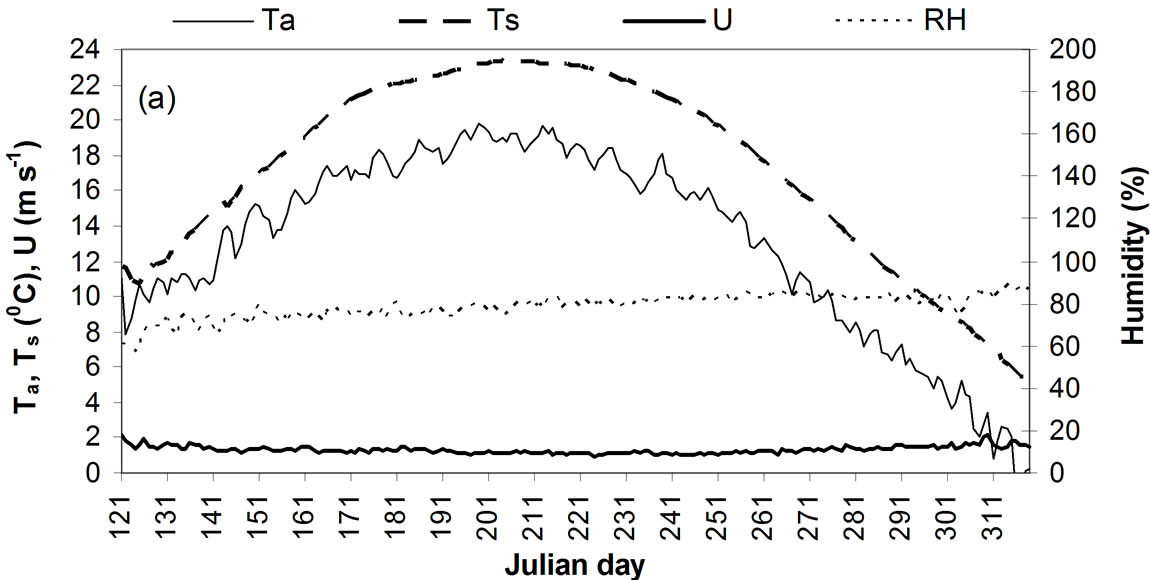
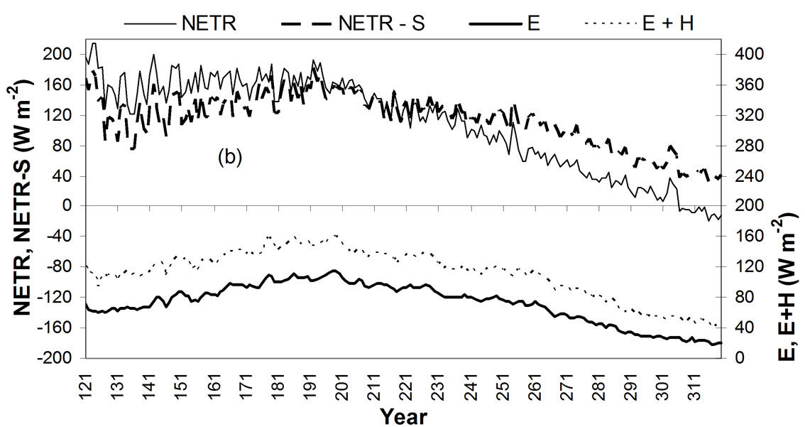
Figure 4. Seasonal changes and patterns of (a) meteorological variable, and (b) energy budget variables, the mean values of daily variables over 30 years.
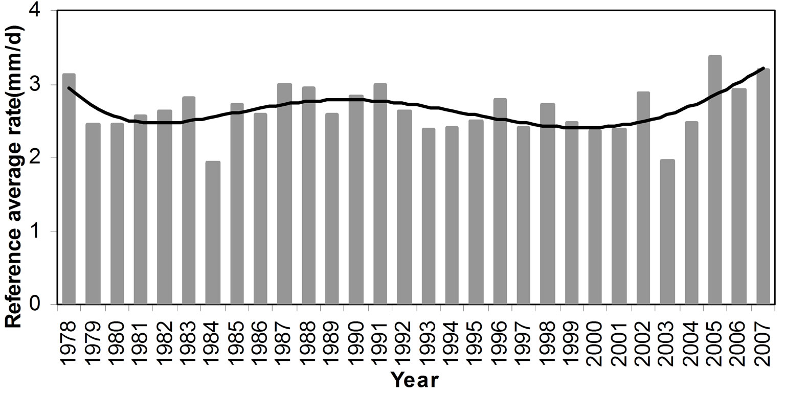
Figure 5. Annual reference evaporation rate averaged over all the days in the span of a year (the bar showing averaged evaporation rate in mm/d, the solid line showing an inter-annual variation pattern of the rates).
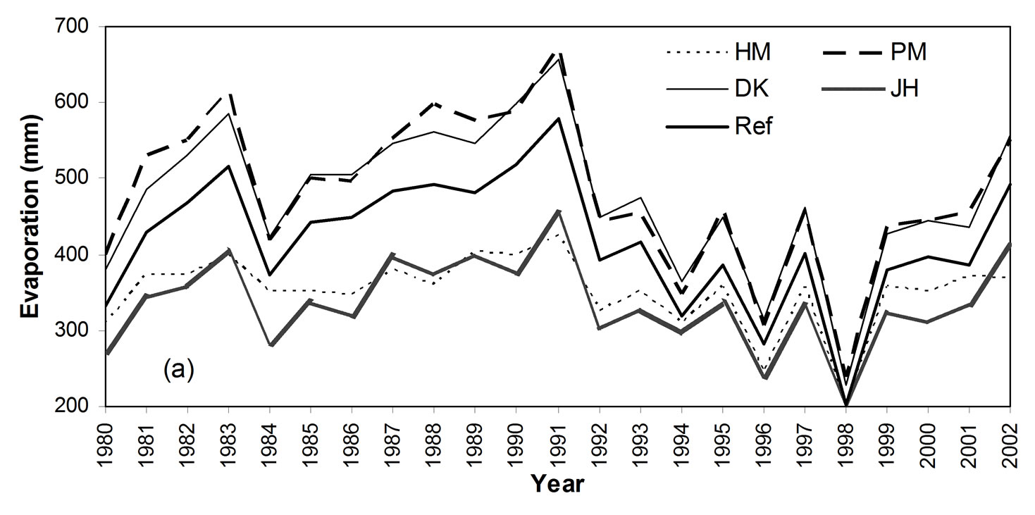

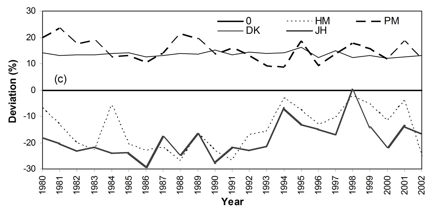
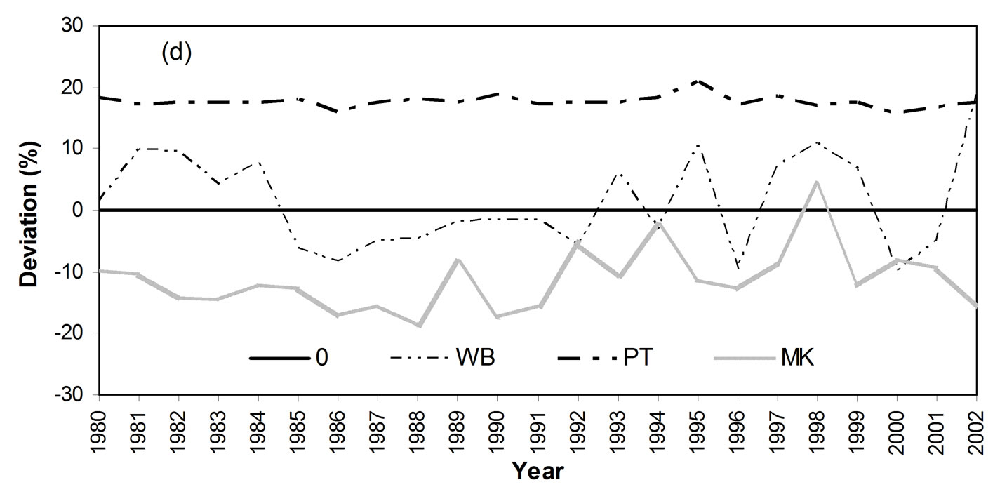
Figure 6. Comparison of method-estimated evaporation with reference evaporation for each of the 30 years: (a) span evaporation (mm) by four methods (HM, PM, DK, JH), (b) span evaporation (mm) by remaining three methods (PT, MK, WB), (c) percent deviation of estimated evaporation from the reference (with HM, PM, DK, JH), and (d) percent deviation of estimated evaporation from the reference (with PT, MK, WB).

Table 3. RMSD and CE values of estimated vs. reference evaporations, and ranked performance of seven evaporation methods when used to span length. The rank of six methods as appeared in Winter et al. study and Rosenberry et al. study are also listed for comparison.
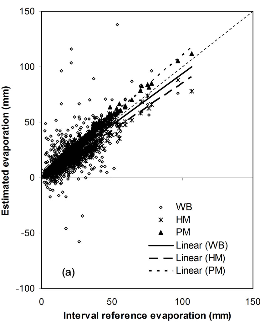
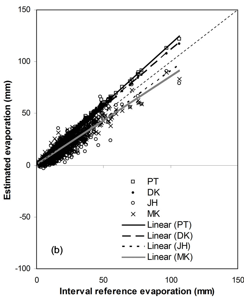
Figure 7. Comparison of interval evaporations against the reference: (a) evaporations from WB, HM and PM and their linear trends, (b) evaporations from PT, DK, JH and MK and their trends.

Table 4. RMSD and CE values and ranked performance of seven methods when used to interval evaporation.
4.2. Evaporation from Seven Methods and Method Comparison
Among the seven methods, six provide evaporation estimations for 30 years (1978–2007): Hamon (HM), Penman (PM), Priestley-Taylor (PT), DeBruin-Kejiman (DK), Jensen-Haise (JH) and Makkink (MK), as they rely on meteorological data. The water balance (WB) provides estimations for 23 years (1980–2002) because the lake level observation data is available only for these years. Therefore, the results from these 23 years are presented and used for comparison. Estimated evaporations in annual spans are shown in Figure 6. The results are divided into two groups in the figure to provide a better distinguishing, as all results plotted on one figure would make the lines difficult to be distinguished. One group includes four methods: HM, PM, DK and JH, the other group includes three methods: PT, MK and WB. Results of evaporation obtained from the seven methods and the reference evaporation from energy budget are shown in Figure 6(a) and (b). Evaporations from WB are mostly close to reference evaporations, results of Penman, Priestley-Taylor, DeBruin-Kejiman and Makkink methods are away from the reference, whereas results of Hamon and Jensen-Haise are even farther from the reference.
Another feature that is seen from Figure 6(a) and (b) is the inter-annual change. Except for the Hamon method, evaporations of the other six methods have almost identical changing patterns: very low in 1984 and 1998, very high in 1983, 1991 and 2002. The major reason for this similarity is that they use a controlling meteorological factor – solar radiation which has had the inter-annual change. The Hamon uses only air temperature which does not show such a change style.
The percent deviations (or errors) of method-estimated evaporation from the reference evaporation are shown in Figure 6(c) and (d). The WB deviations are scattered around the zero level (zero error level), with both positive and negative errors, being the best evenly scattered over the 23 years. The PM or PT or DK deviations are scattered above the zero level (over estimated) for all 23 years. The overestimation of Penman and Priestley-Taylor methods are often reported [9]. The HM, JH and MK deviations are scattered below the zero level (under estimated) for all years except for 1998.
Values of root mean squared deviation (RMSD) between estimated and reference span evaporation, and values of coefficient of efficiency (CE) are listed in Table 3. A lower RMSD value or a higher CE value indicates a lower error between the estimated and observed evaporation, i.e. a better performance in evaporation calculation. Therefore, a performance rank from best to least is determined by the RMSD and CE values, and the rank is: WB, MK, DK, PM, PT, HM, and JH.
Method comparison results with regards to span evaporation might differ from a comparison using interval evaporation. The estimated evaporations for 490 intervals in the 23 years are illustrated in Figure 7 against their corresponding reference evaporations, with three methods in Figure 7(a) and other four methods in Figure 7(b). A linear trend line is shown for each method’s result, and the slope 1:1 center line is also drawn. Surprisingly, the results from WB scattered greatly around the center line, indicating the worst result (opposite to being the best result with the span comparison), although its trend is mostly close to the center line. Method PM, PT and DK tend to overestimate evaporations, while method HM, JH and MK tend to underestimate evaporations.
Similarly to span comparison, the RMSD and CE values of estimated interval evaporation vs. the reference are summarized in Table 4. The rank is: DK, PM, PT, MK, HM, JH and WB. The performance and ranking of seven methods, when applied to estimate evaporation in shorter time duration, are different from the performance when applied to estimate evaporation in longer duration.
Why the water balance calculations do not give reliable evaporations for intervals? When the time duration becomes shorter, the magnitude of evaporation item becomes smaller in the water balance items (compared to precipitation, runoff, outflow, lake level change), and influence of data mistakes or observation uncertainties become more obvious. For instance, if the evaporation is in a magnitude of 30 mm for an interval of 10 days, then any single mistake in lake level, precipitation or discharge could reach to 5 mm, and the mistake could cause a 17% influence on evaporation through water balance accounting. Combined influence of multiple mistakes could cause severer error in evaporation result. But for an evaporation of 500 mm in a span of 7 months, the influence of the same mistake would be 1%.
Collectively assessing Table 3 and Table 4, it is noted that the method HM and JH perform comparatively worse in both cases of span and interval, and should be avoided if other methods are applicable. The DK, MK, PM and PT perform either the best or better than other methods in both cases, and therefore should be well applied to lake evaporation calculation. The water balance WB can be satisfactorily used to long duration (annual, open water season), but should not be used to short duration (weeks, month).
5. Discussion
There may be concerns about the collection location of meteorological data or the distance of the weather station to the lake. Our data are from a station located approximately 1.0 km away from Dickie Lake, not from a raft facility on the lake. This concern was addressed by the study results of Winter et al. [23]. They used 11 evaporation methods including six we used here, and they compared the differences caused by using raft-based, land-based (near the lake) and remote-site-based (60 km away) data. Their results indicated that the usage of raftand land-based data did not result in marked differences in evaporation rates for those six methods. Therefore, the location of our meteorology station on land instead of on lake is not a concern, although raft-based data would have been desirable.
As indicated before, the energy-budget equations only calculated a total evaporation amount within a period because of limited number of lake temperature profiles, and the daily evaporation rate in the period was allocated by using daily rates estimated from the Hamon formula. These allocated daily evaporations used as reference rates could contain potential errors associated with the allocation, since Hamon formula only utilized air temperature and could have large bias from true evaporation rate. Two rational are suggested to argue for the daily allocation. Method comparison in the study was made on the basis of annual span evaporation or interval evaporation, not daily rates. The high accuracy of energy-budget results for periods and spans have been ensured by the method itself. Secondly, although the Hamon evaporation amount for a period might be less accurate than that of energy budget, the distribution pattern of daily rates within the period is usually similar between the two methods. The similar distribution is used to allocate daily rates for energy budget method. Resulted daily rates would not be exactly the same as the values that would be calculated on daily basis if there were available water temperature data, however, the resulted rates should be quite close to those values.
The performance rank of the six methods (not including WB) recommended by Winter et al. [23] and the rank of same six methods recommended by Rosenberry et al. [14] are also listed in Table 3. It would be understandable that the three ranks may be different because the lakes are in different locations, and the datasets used are different. However, the three ranks are similar to some extent. DeBruin-Kejiman and Penman are among the better methods, with DK being the 3rd position among all three ranks; Hamon and Jensen-Haise are among those showing poorer results, positioned at 6th and 7th among all ranks. If comparing two ranks, the difference between our rank and Winter rank is that Makkink, DeBruin-Kejiman and Penman are positioned at 2, 3 and 4 in our rank, against 4, 3 and 2 in Winter rank. The difference between our rank and Rosenberry rank is that Makkink and Priestley-Taylor are positioned at 2 and 5 in our rank, against 5 and 2 in Rosenberry rank. In other words, it is more possible and reliable to use an evaporation method from the energy-aerodynamics combination group, such as Penman, DeBruin-Kejiman and Priestely-Taylor. A method from the two-parameter (solar radiation and temperature) group, such as Makkink, may provide a satisfactory estimation of lake evaporation. But a method from the temperature-only group, such as Hamon, provides poorer estimations.
An effort is tried to interpret physical or logic reasons to why the methods perform in a way as shown in Table 3, why some methods perform better than other ones. First of all the accuracy of the reference method – energy budget would not be doubted, as it is based on strictly-defined theories and has been proved by many researchers. It provides reliable evaporation reference provided that the input data are correctly collected. The best performer – water balance method (Equation (16)) has the ability to provide good evaporation estimations, if the in and out items are well measured. The runoff coming from 2/3 watershed area of Dickie Lake has been well monitored, precipitation and outflow are well monitored too, and lake level is measured too. This data information ensures that estimated evaporation in spans is reasonable and reliable. The second-ranked Makkink method (Equation (15)) has a simple empirical format and uses only air temperature and short-wave radiation as input. These two factors are the most important among many meteorological factors. Its equation has a fairly correct description of the two key factors, and the equation applies well to the lake in the Canadian Shield as it did to its original datasets. Although it gives fairly good evaporation estimates, it has a drawback of underestimation. Probably a minor adjustment to the equation (i.e. change the constant 0.61) can improve this drawback.
The third-ranked DeBruin-Kejiman method is an empirical equation similar to Makkink, considers more affecting factors (temperature, shortand long-wave radiations, lake heat storage) than MK does. Its performance is accepted just because it can be applied to the studied lake without equation adaption. Actually the overestimation problem as seen from Figure 6 could be improved by adjusting the equation. The fourth-ranked Penman method (Equation (10)) has been widely used to estimate lake evaporation or watershed potential evapotranspiration, having taken consideration of all affecting factors. There might be two reasons leading to its overestimation problem: the function in relation to the wind speed and the period-averaging treatments in wind speed and air humidity. The fifth-ranked Priestley-Taylor method (Equation (12)) is an empirical equation similar to DK. Its not-good performance means that probably it needs adjustment to be well applied to the study area, for example changing its constant 1.26. One common concern for the three methods (DK, PM, PT) which all overestimate evaporation is noted but has not been identified: they all include a net radiation in their equations. If the net radiation were not correctly measured or calculated, a systematic overestimation would have occurred.
The sixth-ranked Hamon method (Equation (8)) does not give good estimates simply because it only considers air temperature as the controlling factor. Unless the meteorological data is severely restricted, this method is not recommended for lake evaporation. The seventh-ranked Jensen-Haise method (Equation (14)) includes very sitedependent parameters, and may be not applicable to our study lake without proper adjustment. The evaporation is badly underestimated.
The data length of 30 years would remind that a timely trend analysis may be worthwhile. All meteorological and energy budget variables were checked to find potential trends or periodic cycles in the 30 years, but none has been found to have a significant trend at Dickie Lake. Linacre [40] proposed that lake-evaporation rate is generally decreasing at around 0.1 mm/d per decade around the world, chiefly on account of reduced solar radiation. The estimated rates by energy budget method for Dickie Lake do not show such a reduction. The averaged daily rate in ice-free season for three decades (1981–1990, 1991–2000, 2001-2007, with the third decade being 7 years only) is 2.66, 2.57 and 2.74 mm/d respectively, the rate decreases by 0.09 mm/d from the first to second decade, but increases 0.17 mm/d from the second to third decade.
Apart from the traditional methods such as the energy budget and seven methods used here that need meteorological data, a newer way to estimate lake evaporation is by using isotope technology. Saxena [41] estimated evaporation from a central Swedish lake by measuring oxygen-18 content in lake water, stream inflows and outflow, and precipitation. The results of isotope method were further compared with results of bulk-aerodynamic and Bowen ratio methods [42]. Except for some situations such as high-precipitation events, high-outflow periods or rapid lake-volume change periods, the evaporation estimated from the three methods agreed. A similar experimental study was conducted by He et al. (personal correspondence with one of the authors, 2009) for Dickie Lake by measuring oxygen-18, and their results gave a total evaporation 660 mm for year 2003 (January 1 to December 31). For comparison, a total evaporation for the same year was calculated using the Makkink method (it needed air temperature and radiation data, not needing lake temperature), and the calculated evaporation was 451 mm. This reveals a significant difference between isotopeestimated evaporation and Makkink-estimated evaporation.
6. Conclusions
The 30 year dataset from Dickie Lake provided a valuable opportunity to conduct a long-term study on lake evaporation. Evaporations in longer spans and shorter intervals during ice-free season were calculated separately using seven evaporation methods, based on field meteorology, hydrology and lake water temperature data. A reference value of the evaporation was provided by a lake water energy budget, and was used to evaluate the performance of the seven methods. The deviations of method-induced evaporation from reference evaporation were compared among the seven methods, and a performance rank was proposed based on the comparison. For purpose of evaporation in long time duration such as a span or a year, the best-to-least methods were ranked as: water balance, Makkink, DeBruin-Kejiman, Penman, Priestley-Taylor, Hamon, and Jensen-Haise. For purpose of evaporation in short time such as an interval or a month, the best-to-least methods were ranked as: DK, PM, PT, MK, HM, JH and WB. Overall, four methods (MK, DK, PM and PT) work better than other three methods.
Details of energy budget, correspondences between energy terms and meteorological variables, annual or seasonal changes of these terms and variables, and the compensation function of lake heat storage in evaporation flux were also analyzed and illustrated. Within the ice-free duration of a year, lake water absorbed a portion of net radiation in early and mid summer, and released the absorbed energy in the fall to compensate for evaporation. Strong correspondence existed between net radiation and consumptive heat flux (latent and sensible heat) but with a time lag, or between temperature and the heat flux. From year to year, the lake heat storage did not play a notable role in energy budgeting, and lake evaporation or consumptive heat flux was controlled by the net radiation. Our study results have shown a similar energy budget pattern as other studies in similar climatic regions, and identified a performance rank for the evaporation calculation methods to be used for lakes in Canadian Shield.
7. Acknowledgements
The author would like to thank Robert Girard for his assistance in lake morphometry and profile data, and thank Joe Findeis and Ron Ingram for their assistance in meteorology data. Thank Peter Dillon, Lance Aspden and Christiane Guay for their discussion and comment. Numerous former governmental staff and university partners have contributed to the data collection and management.
REFERENCES
- G. Krantzberg, “The Great Lakes, a 35th year anniversary: Time to look forward,” Electronic Green Journal, Vol. 26, pp. 1–4, 2008.
- N. D. Yan, A. M. Paterson, K. M. Somers, and W. A. Scheider, “An introduction to the Dorset special issue: transforming understanding of factors that regulate aquatic ecosystems on the southern Canadian Shield,” Canadian Journal of Fisheries and Aquatic Sciences, Vol. 65, pp. 781–785, 2008.
- J. J. Gibson and W. D. Edwards, “Regional water balance trends and evaporation-transpiration portioning from a stable isotope survey of lakes in northern Canada,” Global Biogeochemical Cycles, Vol. 16, No. 10, pp. 1–14, 2002.
- Minnesota DNR Waters, “Lake-ground water interaction study at White Bear Lake, Minnesota,” Minnesota Department of Natural Resources Report, Minnesota, USA, 1998.
- G. Weyhenmeyer, “Rates of change in physical and chemical lake variables – are they comparable between large and small lakes?” Hydrobiologia, Vol. 599, pp. 105–110, 2008.
- J. D. Lenters, T. K. Kratz, and C. J. Bowser, “Effects of climate variability on lake evaporation: Results from a long-term energy budget study of Sparkling Lake, northern Wisconsin (USA),” Journal of Hydrology, Vol. 308, pp. 168–195, 2005.
- J. J. Gibson, R. Reid, and C. Spence, “A six-year isotopic record of lake evaporation at a mine site in the Canadian subarctic: Results and validation,” Hydrological Processes, Vol. 12, pp. 1779–1792, 1998.
- Y. Mahrer and S. Assouline, “Evaporation from Lake Kinneret, 2. Estimaton of the horizontal variability using a two-dimensional numerical mesoscale model,” Water Resources Research, Vol. 29, pp. 911–916, 1993.
- W. Abtew, “Evaporation estimation for Lake Okeechobee in South Florida,” Journal of Irrigation and Drainage Engineering, Vol. 127, pp. 140–147, 2001.
- R. J. Dos Reis and N. L. Dias, “Multi-season lake evaporation: energy-budget estimates and CRLE model assessment with limited meteorological observations,” Journal of Hydrology, Vol. 208, pp. 135–147, 1998.
- U.S. Geological Survey, “Estimating Evaporation from Lake Mead,” USGS Scientific Investigations Report, No. 2006-5252, Arizona, USA, 2006.
- J. A. Amayreh, “Lake evaporation: a model study,” in Dissertation Abstracts International 57-03, Section B, Utah State University, pp. 1938, 1995.
- D. O. Rosenberry, D. I. Stannard, T. C. Winter, and M. L. Martinez, “Comparison of 13 equations for determining evapotranspiration from a prairie wetland, Cottonwood Lake Area, North Dakota, USA,” Wetlands, Vol. 24, pp. 483–497, 2004.
- D. O. Rosenberry, T. C. Winter, D. C. Buso, and G. E. Likens, “Comparison of 15 evaporation methods applied to a small mountain lake in the northeastern USA,” Journal of Hydrology, Vol. 340, pp. 149–166, 2007.
- E. Robertson and P. J. Barry, “The water and energy balances of Perch Lake (1969–1980),” Atmosphere-Ocean, Vol. 23, pp. 238–253, 1985.
- A. H. Rasmussen, M. Hondzo, and H. G. Stefan, “A test of several evaporation equations for water temperature simulations in lakes,” Water Resources Bulletin, Vol. 31, pp. 1023–1028, 1995.
- P. F. Hamblin, H. A. Bootsma, and R. E. Hecky, “Surface meteorological observations over Lake Malawi/Nyasa,” Journal of Great Lakes Research, Vol. 29, pp. 19–23, 2003.
- M. E. Keskin and O. Terzi, “Evaporation estimation models for Lake Egirdir, Turkey,” Hydrological Processes, Vol. 20, pp. 2381–2391, 2006.
- E. T. Linacre, “Data-sparse estimation of lake evaporation, using a simplified Penman equation,” Agricultural and Forest Meteorology, Vol. 64, pp. 237–256, 1993.
- W. A. Scheider, R. A. Reid, B. A. Locke, and L. D. Scott, “Studies of lakes and watersheds in Muskoka-Haliburton, Ontario: Methodology (1976–1982),” Data Report DR 83/1 of Ontario Ministry of the Environment, Dorset, Ontario, Canada, 1983.
- W. A. Scheider, C. M. Cox, and L. D. Scott, “Hydrological data for lakes and watersheds in Muskoka-Haliburton study area (1976–1980),” Data Report DR 83/6 of Ontario Ministry of the Environment, Dorset, Ontario, Canada, 1983.
- B. A. Hutchinson, L. D. Scott, M. N. Futter, and A. Morgan, “Hydrology data for lakes and catchments in Muskoka/Haliburton (1980–1992),” Data Report DR 93/2 of Ontario Ministry of the Environment, Dorset, Ontario, Canada, 1994.
- T. C. Winter, D. O. Rosenberry, and A. M. Sturrock, “Evaluation of 11 equations for determining evaporation fro a small lake in the north central United States,” Water Resources Research, Vol. 31, pp. 983–993, 1995.
- M. S. Mosner and B. T. Aulenbach, “Comparison of methods used to estimate lake evaporation for a water budget of Lake Semnole, southwestern Georgia and northwestern Florida,” in Proceedings of the 2003 Georgia Water Resources Conference, Athens, Georgia, USA, 2003.
- C.-Y. Xu and V. P. Singh, “Evaluation and generalization of radiation-based methods for calculating evaporation,” Hydrological Processes, Vol. 14, pp. 339–349, 2000.
- V. P. Singh and C.-Y. Xu, “Evaluation and generalization of 13 mass-transfer equations for determining free water evaporation,” Hydrological Processes, Vol. 11, pp. 311– 323, 1997.
- F. Delclaux, A. Coudrain, and T. Condom, “Evaporation estimation on Lake Titicaca: a synthesis review and modelling,” Hydrological Processes, Vol. 21, pp. 1664–1677, 2007.
- M. F. Sadek, M. M. Shahin, and C. L. Stigter, “Evaporation from the reservoir of the High Aswan Dam, Egypt: A new comparison of relevant methods with limited data,” Theoretical and Applied Climatology, Vol. 56, pp. 57–66, 1997.
- R. A. Reid, R. Girard, and A. C. Nicolls, “Morphometry and catchment areas for the calibrated watersheds,” Data Report DR 87/4 of Ontario Ministry of the Environment, Dorset, Ontario, Canada, 1987.
- V. T. Chow, D. R. Maidment, and L. W. Mays, “Applied hydrology,” McGraw-Hill Book Company, New York, 1988.
- A. L. Buck, “New equations for computing vapour pressure and enhancement factor,” Journal of Applied Meteorology, Vol. 20, pp. 1527–1532, 1981.
- H. Yao and I. F. Creed, “Determining spatially-distributed annual water balances for ungauged locations on Shikoku Island, Japan: a comparison of two interpolators,” Hydrological Sciences Journal, Vol. 50, pp. 245–263, 2005.
- J. Doorenbus and W. O. Pruitt, “Guidelines for predicting crop water requirements”, Irrigation and Drainage Paper No. 24, Food and Agriculture Organization of the United Nations, Rome, Italy, 1977.
- H. Yao, A. Terakawa, and S. Chen, “Rice water use and response to potential climate changes: calculation and application to Jianghan, China,” in Proceedings of the International Conference on Water Resources and Environment Research , Kyoto, Japan, Vol. 2, pp. 611–618, 1996.
- H. A. R. DeBruin and J. Q. Kejiman, “The Priestley-Taylor evaporation model applied to a large, shallow lake in the Netherlands,” Journal of Allied Meteorology, Vol. 18, pp. 898–903, 1979.
- K. J. Devito and P. Dillon, “Errors in estimating stream discharge in small headwater catchments: influence on interpretation of catchment yields and input – output budget estimates,” Technical Report 1993 of Ontario Ministry of the Environment, Dorset, Ontario, Canada, 1993.
- S. W. Hostetler and P. J. Bartlein, “Simulation of lake evaporation with application to modeling lake level variations of Harney-Malheur Lake, Oregon,” Water Resources Research, Vol. 26, pp. 2603–2612, 1990.
- N. G. Grannemann, R. J. Hunt, J. R. Nicholas, T. E. Reilly, and T. C. Winter, “The importance of ground water in the Great Lakes region,” Water-Resources Investigation Report 00-4008, U. S. Geological Survey, Lansing, Michigan, 2000.
- J. E. Nash and J. V. Sutcliffe, “River flow forecasting through conceptual models: Part I – a discussion of principles,” Journal of Hydrology, Vol. 10, pp. 282–290, 1970.
- E. T. Linacre, “Evaporation trends,” Theoretical and Applied Climatology, Vol. 79, pp. 11–21, 2004.
- R. K. Saxena, “Estimation of lake evaporation from a shallow lake in central Sweden by oxygen-18,” Hydrological Processes, Vol. 10, pp. 1273–1281, 1998.
- R. K. Saxena, C. Jaedicke, and L. C. Lundin, “Comparison mass-balance, bulk aerodynamic and bowen ratio methods,” Physics and Chemistry of the Earth, Part B: Hydrology, Oceans and Atmosphere, Vol. 24, pp. 851– 859, 1999.