Journal of Software Engineering and Applications
Vol.5 No.4(2012), Article ID:18568,8 pages DOI:10.4236/jsea.2012.54027
Additive Fault Tolerant Control Applied to Delayed Singularly Perturbed System
![]()
1Research Unit Modeling, Analysis and Control Systems (MACS), Gabes, Tunisia; 2National Engineering School of Gabes, Gabes, Tunisia; 3Higher Institute of Technological Studies of Djerba, Djerba, Tunisia.
Email: nouceyba.naceur@laposte.net, Adel Tellili@Lycos.com, naceur.abdelkrim@enig.rnu.tn
Received November 18th, 2011; revised December 20th, 2011; accepted March 13th, 2012
Keywords: Additive Fault Tolerant Control; Composite Control; Lambert W Function; Order Reduction; Sensor Fault; Singularly Perturbed System
ABSTRACT
The additive fault tolerant control (FTC) for delayed system is studied in this work. To design the additive control, two steps are necessary; the first one is the estimation of the sensor fault amplitude using a Luenberger observer with delay, and the second one consists to generate the additive fault tolerant control law and to add it to the nominal control of delayed system. The additive control law must be in function of fault term, then, in the absence of fault the expression of additive control equal to zero. The generation of nominal control law consist to determinate the state feedback gain by using the Lambert W method. Around all these control tools, we propose an extension of the additive FTC to delayed singularly perturbed systems (SPS). So, this extension consists to decompose the delayed SPS in two parts: delayed slow subsystem (delayed SS) and fast subsystem (FS) without time delay. Next, we consider that the delayed SPS is affected at its steady-state, and we apply the principal of FTC to the delayed SS and finally we combine them with the feedback gain control of FS by using the principal of composite control.
1. Introduction
Several physical processes are on one hand high order and on the other hand are complex what returns their analysis and especially their control, with the aim of certain objectives, very delicate. However, knowing that these systems possess variables evolving in various speeds (temperature, pressure, intensity, voltage…) it turned out interesting to separate their dynamics [1-6] with the aim of the implementation of singularly perturbation technique. Indeed, this one allows, in the case of two time scales, [7] to describe the behavior of global studied process by those of two their subsystem (slow and fast) obtained by a temporal decomposition.
The interest of this decomposition is to define a reduced order model which allows in several control problems to found a solution simpler to implement for some approximations.
Like for all the types of systems who can contain a time-delay in its dynamic or in their control, the singularly perturbed systems “SPS” can also contain a delay. This problem was studied in several references such as [8-12], etc.
Moreover the presence of fault in delayed SPS complicate their designs for this reason it’s necessary to elaborate a fault tolerant control FTC.
This paper is the extension of the additive fault tolerant control designed for the SPS in [13] to the delayed SPS case and it’s the extension of additive FTC in [14, 15] to the delayed systems and specially to the delayed singularly perturbed system.
2. Delayed Singularly Perturbed System
Consider the standard linear singularly perturbed system with small state time-delay described by [16,9]:
Delayed SPS
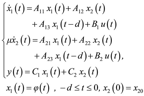 (1)
(1)
where: 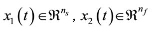 are the states vector,
  the control input, d the positive time-delay, μ the small positive perturbation parameter Aij, Bi, i = 1, 2; j = 1, 2, 3, constant matrices of appropriate dimensions, and φ(t) the continuously differentiable initial function.
The slow subsystem (SS) and fast subsystem (FS) are obtained by considering that the fast variable in x2(t) reached there established regime, which corresponds to the assumption μ = 0 [2,17]. This leads then to the following reduced models:
Delayed SS
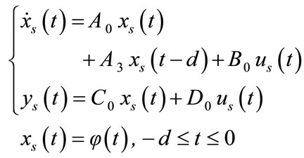 (2)
(2)
with:
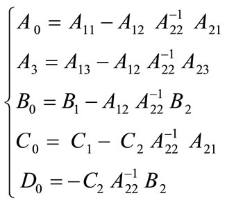 (3)
(3)
and FS
 (4)
(4)
3. Principle of Additive Fault Tolerant Control
The accommodation principle of fault is based on the addition of an additive control uad to the nominal control law u. To design this control law, we need two steps: estimation and compensation of the fault.
In our work we studied only the sensor fault case which appears as bias. In this section we will consider that the delayed SPS is affected at its steady-state, so that it is equivalent to consider that the fault affects only the delayed slow subsystem and by consequence we will design only the reduced additive FTC of slow subsystem and the additive control of delayed slow subsystem will be applied to delayed SPS to compensate its sensor fault. The first step consists to design nominal composite control for the delayed SPS, secondly the sensor fault amplitude will be estimated by using the delayed slow subsystem, and finally we determinate the expression of reduced additive FTC.
3.1. Composite Nominal Control
This approach was developed for the SPS without timedelay in [1,7,13]. The results will be extended it to the delayed SPS. Its principle consists to determinate the state feedback gain of slow subsystem and of fast subsystem, the last ones will be regrouped to find a global gain of SPS.
We remark that the delayed SPS is decomposed in delayed slow subsystem and fast subsystem without timedelay, for this reason we will design the state feedback gain of slow subsystem by using the Lambert-W function and the state feedback gain of fast subsystem will be determinate by using the classical pole placement method.
3.1.1. Determination of Reduced Nominal Control of Delayed Slow Subsystem
The Gain of slow subsystem control is determined by using the Lambert-W approach.
Definition of Lambert W function:
Let’s  be a solution, to determinate, of the equation
 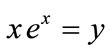 for
for , This type of equation can be resolve by using the Lambert W function
  such that [18,19]:
 .
.
With: k branches of Lambert W function and k є [−∞, +∞], k = 0 principal branch [18,19].
Consider the delayed system:
 (5)
(5)
This can be represented by the delayed differential equation (DDE):
 (6)
(6)
Let’s 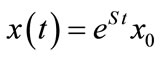 be a solution of (6) with S: matrix, with appropriate dimension, to determinate.
Replacing the expression of  in (6) we find:
 (7)
(7)
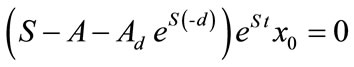
By consequence we found:
 (8)
(8)
Then:
 (9)
(9)
Multiplying the Equation (9) by  we find:
 (10)
(10)
In this step we can use Lambert W function with  and
and , by consequence the expression of S is:
 (11)
(11)
Equation (11) represents the characteristic equation for the general time-delayed system [20]. The roots of Equation (6) are the eigenvalues of the matrix S and can be used to describe the stability of the DDE (6), which represents the stability of the general system.
State feedback gain of slow subsystem by using Lambert W function
Consider the feedback control of delayed slow subsystem:
 (12)
(12)
To find  we place the desired eigenvalue as follow:
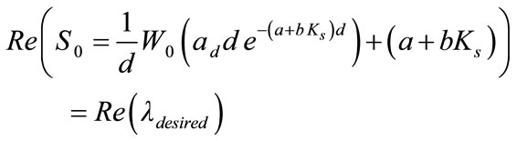 (13)
(13)
We consider, also, that the slow subsystem is augmented by an integrator to ensure a null static error. So, the expression (12) of Reduced will be:
 (14)
(14)
where: 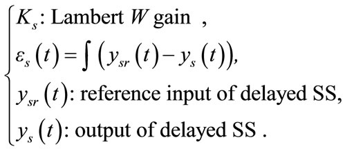
The expression of delayed slow subsystem in closed loop is:
 (15)
(15)
with: ,
, 
3.1.2. Gain State Feedback of Fast Subsystem
The Gain of fast subsystem control is determined by using the classical placement pole method.
 (16)
(16)
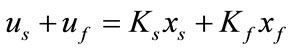
3.1.3. Composite State Feedback Control of SPS
The composite nominal control of SPS is determinate by regrouping the two gains of delayed slow subsystem and fast subsystem.
View on the composite control of SPS without timedelay
Consider the form of slow subsystem and fast subsystem control represented by the two Equations (12) and (16), the composite control can be determinate by using the following equation [1,7]:
 (17)
(17)
However, the composite control law must be expressed using the system states x1 and x2, this can be obtained by replacing xs by x1 and xf by x2 – x2s ,with:  and x2s is the slow part of x2.
By consequence, the composite control law is:
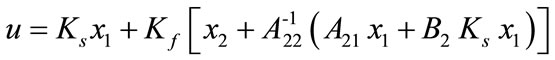 (18)
(18)
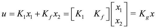 (19)
(19)
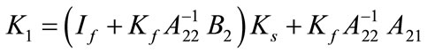 (20)
(20)
Composite control of delayed SPS
The composite control gain of delayed SPS is determinate by analogy of non-delayed case of SPS, and as shown in Figure 1 the composite nominal control  of delayed SPS is:
 (21)
(21)
with: 
3.2. Additive Control Law
We suppose that the SPS is affected by a sensor fault in its steady-state. Given that the SPS output in steady-state is approximated by the one of slow subsystem; we can estimate the fault amplitude affecting the SPS by using the delayed slow subsystem.
The main goal in this part is the determination of reduced additive control by using the delayed slow subsystem in order to compensate the sensor fault affecting the global delayed SPS.
Figure 2 represents the principle of Fault tolerant control of delayed SPS.
3.2.1. Fault Amplitude Estimation
This step is realized by using the delayed Luenberger observer represented by the following equation:
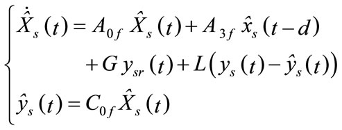 (22)
(22)
with:

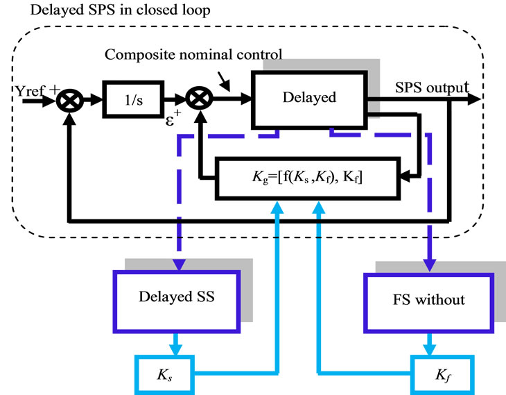
Figure 1. Principle of composite nominal control of delayed SPS.

Figure 2. Principle of fault tolerant control of delayed SPS.
The dynamic of observation error is:
 (23)
(23)
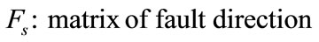
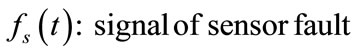
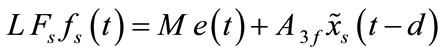
The output of delayed slow subsystem affected by sensor fault is:
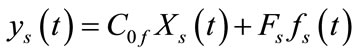 (24)
(24)
Using the Equations (15), (22) and (24) the expression of  becomes:
 (25)
(25)
with: 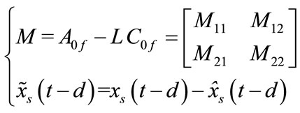
In steady-state the estimation error becomes null  then via (25) we can find the expression of fault amplitude:
 (26)
(26)
Knowing that Fs is scalar and L is the observer gain of augmented system (dim (L) =2 × 1 and ) then (L Fs) is not invertible and by consequence we decompose the Equation (26).
So, the expression of fault is:
 (27)
(27)
with: 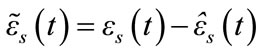
3.2.2. Determination of Reduced Additive Control of Delayed Slow Subsystem
The compensation of sensor fault effect on the closedloop system can be achieved by adding a new control law to the nominal one [14,15]:
 (28)
(28)
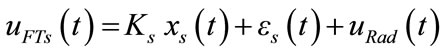
The output and the integrator are affected with the fault such that:
 (29)
(29)
If C0 = 1 and by using Equations (28) and (29), the control law becomes the follow expression:
 (30)
(30)
The effect of sensor fault can be compensated by using the additive control as follow:
 (31)
(31)
3.2.3. Determination of Global Additive Control of Delayed SPS
We can deduce the expression of global additive control of delayed SPS by adding the reduced additive control (31) to the composite nominal control defined by expression (21):
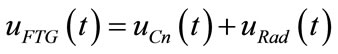 (32)
(32)
4. Simulation Example
Consider the delayed SPS:
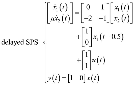
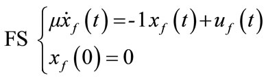
If μ tends toward zero we find the delayed slow subsystem and the fast subsystem:

By using the Equation (13), “lambertw” function in MATLAB and by placing the desired pole equal (- 2.1), we find Ks = –1.5;
So, the reduced control is .
.
The gain Kf = –0.1 is determined by using expression (16).
By regrouping the two gains and using the expression (20) and (21) we find the following composite nominal control of SPS: 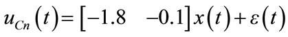
The gain of observer is determined by placing the poles of  such as the eigenvalues of
  equals 40 times the eigenvalues of
 , so
, so
 .
.
So, the fault tolerant control of delayed SPS as show the expression (32) is:

To simulate the effect of the fault tolerant control we generate a sensor fault as bias at time t = 40 sec with amplitude equal 0.5;
The following Figures 3(a) and (b) show the effect of sensor fault respectively in the control and in the output, of delayed SPS and delayed slow subsystem.
The estimation of the sensor fault using the delayed observer is shown in the Figure 4:
Figure 4 shows that the observer can estimate the am-
 (a)
(a)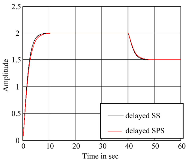 (b)
(b)
Figure 3. (a) Time evolution of controls in the occurrence of sensor fault; (b) Time evolution of outputs in the occurrence of sensor fault.

Figure 4. Sensor fault estimation.
plitude of sensor fault.
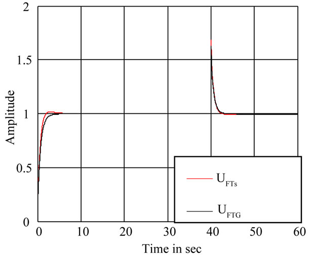
The following Figures 5(a) and (b) show the ability of the fault tolerant control to compensate the effect of sensor fault in the delayed SPS.
 (a)
(a) (b)
(b)
Figure 5. (a) Time evolution of fault tolerant controls; (b) Time evolution of outputs after compensation of sensor fault.
 (a)
(a)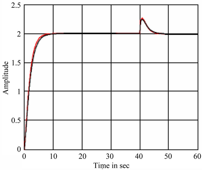 (b)
(b)
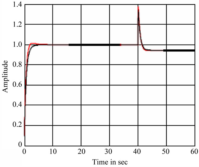
Figure 6. (a) The outputs of delayed SPS and delayed SS for L1; (b) The outputs of delayed SPS and delayed SS for L2.
It’s clear in the Figure 5 that the reduced additive control added to the composite nominal control can compensate the effect of sensor fault in the delayed SPS output.
Effect of observer gain value on the fault compensation
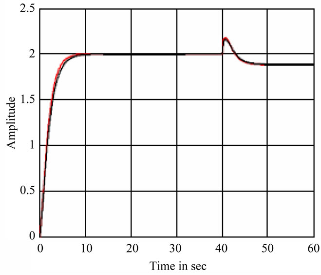
In this paragraph we discuss the effect of observer gain value in the fault compensation error. Figures 6(a) and (b) show the delayed SPS and the delayed SS output for different gain values. Figures 7(a) and (b) represent the control signal for different gain values.
Case (a) for gain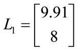 .
.
Case (b) for gain 
It’s clear that for the case (b) the error value is equal to zero, but in case (a) it’s equal to 25% from the amplitude of fault (equal 0.5).
For the case (b) the deviation of control signal at the occurrence of fault (40 sec) is more important than the case (a).
So, more the observer gain value is important, more the compensation error in output of delayed SPS and delayed SS is better but the deviation of control signal is than more important.
5. Conclusions
In this work we studied the fault tolerant control of delayed SPS by using the reduced fault tolerant control based on the delayed slow subsystem. This slow-fast decomposition approach simplifies the design of complex systems control with sensor failure.
We notice an important deviation of the control signal at time of fault occurrence. So it will be interesting to study the fault tolerant control with constraints on the
 (a)
(a) (b)
(b)
Figure 7. (a) The controls of delayed SPS and delayed SS for L1; (b) The controls of delayed SPS and delayed SS for L2.
control signal.
Also, this result can be extended to nonlinear delayed process with other type of faults.
REFERENCES
- P. V. Kokotovic, H. K. Khalil and J. O’Reilly, “Singular Perturbations Method in Control: Analysis and Design,” Academic Press, London, 1986.
- M. N. Abdelkrim, “Sur la Modélisation et la Synthèse des Systèmes Singulièrement Perturbés,” Thèse de Doctorat, de l’Ecole Nationale d’Ingénieurs de Tunis, Tunisie, 1985.
- M. Benrejeb, M. Gasmi and M. N. Abdelkrim, “Nouvelle Méthode de Modélisation des Systèmes Linéaire Singulièrement Perturbés-Méthode du Cercle,” IMACS-IFACSymposium, New Haven, 6-8 August 1986, pp. 569-571.
- M. N. Abdelkrim and M. Benrejeb, “Sur la Sensibilité d’Un modèle Réduit d’un Système Singulièrement Perturbé,” JTEA’9, Monastir, 9-11 December 1988, pp. 1-4.
- F. H. Hasio, S. T. Pan and C. C. Teng, “D-Stability Bound Analysis for Discrete Multiparameter Singularly Perturbed Systems,” IEEE Transactions on Circuit and Systems (I): Fundamental Theory and Applications, Vol. 44, No. 4, 1997, pp. 347-350. doi:10.1109/81.563624
- S.-T. Pan and C.-F. Chen, “Robust Stability Analysis of Discrete Uncertain Singularly Perturbed Time-Delay Systems,” Applied Mathematics Letters, Vol. 19, No. 2, 2006, pp. 197-205. doi:10.1106/j.aml.2005.05.005
- M. S. Mahmoud and M. G. Singh, “Large Scale Systems Modeling,” Pergamon Press, Oxford, 1981.
- E. Fridman, “Stability of Singularly Perturbed Differential-Difference Systems: A LMI Approach,” Dynamics of Continuous, Discrete and Impulsive Systems Series B: Applications & Algorithms, Vol. 9, 2002, pp. 201-212.
- B. L. Zhang and M. Q. Fan, “Near Optimal Control for Singularly Perturbed Systems with Small Time-Delay,” Proceedings of the 7th World Congress on Intelligent Control and Automation, Chongqing, 25-27 June 2008, pp. 7212-7216. doi:10.1109/WCICA.2008.4594039
- L. L. Liu, J. P. Peng and B. W. Wu, “Robust Stability of Singularly Perturbed Systems with State Delays,” Proceedings of the 2009 International Workshop on Information Security and Application (IWISA 2009), Qingdao, 21-22 November 2009, pp. 19-21. doi:10.1049/ip-cta:20030018
- S. T. Pan, C. F. Chen and J.-G. Hsieh, “Stability Analysis for a Class of Singularly Perturbed Systems with Multiple Time Delays,” Transactions of the ASME, Vol. 126, 2004, pp. 462-466.
- N. Abdelkrim, A. Tellili and M. N. Abdelkrim, “Composite Control of a Delayed Singularly Perturbed System by Using Lambert-W Function,” Proceedings of 2010 7th International Multi-Conference on Systems Signals and Devices (SSD), Amman, 27-30 June 2010, pp. 1-4. doi:10.1109/SSD.2010.5585577
- N. Abdelkrim, A. Tellili and M. N. Abdelkrim, “Additive Fault Tolerant Composite State Feedback Control of Singularly Perturbed System,” 6th International Conference on Electrical Systems and Automatic Control, Tunisia, 26-28 March 2010, pp. 26-28.
- H. Noura, “Méthode d’Accommodation aux Défauts: Théories et Applications,” Habilitation à Diriger des Recherches, l’Université Henri Poincaré, Nancy, 2002.
- H. Noura, D. Theilliol, J. C. Ponsart and A. Chamseddine, “Fault-Tolerant Control Systems: Design and Practical Application,” 1st Edition, Springer, Heidelberg, 2009.
- G. Y. Tang, B.-L. Zhang, Y.-D. Zhao and S.-M. Zhang, “Optimal Sinusoidal Disturbances Damping for Singularly Perturbed Systems with Time-Delay,” Journal of Sound and Vibration, Vol. 300, No. 1-2, 2007, pp. 368-378. doi:10.1016/j.jsv.2006.08.034
- A. Tellili, M. N. Abdelkrim and M. Benrejeb, “Model Based Fault Diagnosis of Two-Time Scales Singularly Perturbed Systems,” Proceedings of 2004 First International Symposium on Control, Communications and Signal, Hammamet, 21-24 March 2004, pp. 819-822. doi:10.1109/ISCCSP.2004.1296571
- Y. Sun, P. W. Nelson and A. G. Ulsoy, “Feedback Control via Eigenvalues Assignment for Time Delayed Systems Using the Lambert W Function,” Proceedings of the ASME 2007 International Design Engineering Technical Conferences & Computers and Information in Engineering Conference (IDETC/CIE 2007), Las Vegas, 4-7 September 2007, pp. 783-792. doi:10.1115/DETC2007-35711
- Y. Sun and A. G. Ulsoy, “Solution of a System of Linear Delay Differential, Equations Using the Matrix Lambert Function,” Proceedings of the 2006 Conference on American Control, Minneapolis, 14-16 June 2006, p. 6. doi:10.1109/ACC.2006.1656585
- K. M. Pietarila and F. Roger, “Developing and Automating Time Delay System Stability Analysis of Dynamic Systems Using the Matrix Lambert W (MLW) Function Method,” Ph.D. Thesis, University of Missouri, Columbia, 2009.