Natural Science
Vol.4 No.3(2012), Article ID:18064,10 pages DOI:10.4236/ns.2012.43022
Modeling geologically abrupt climate changes in the Miocene: Potential effects of high-latitudinal salinity changes
![]()
1EMS Earth and Environmental Systems Institute, Pennsylvania State University, University Park, USA; *Corresponding Author: bjhaupt@psu.edu
2NOAA/National Oceanographic Data Center, Silver Spring, USA
Received 7 January 2012; revised 10 February 2012; accepted 26 February 2012
Keywords: Cenozoic; Miocene; palao-climate modeling; Community Climate Model 3.6; Modular Ocean Model 2.2; meridional overturning; freshwater balance; high-latitudinal salinity changes
ABSTRACT
The cooling of the Cenozoic, including the Miocene epoch, was punctuated by many geologically abrupt warming and cooling episodes— strong deviations from the cooling trend with time span of ten to hundred thousands of years. Our working hypothesis is that some of those warming episodes at least partially might have been caused by dynamics of the Antarctic Ice Sheet, which, in turn, might have caused strong changes of sea surface salinity in the Miocene Southern Ocean. Feasibility of this hypothesis is explored in a series of offline-coupled oceanatmosphere computer experiments. The results suggest that relatively small and geologically short-lived changes in freshwater balance in the Southern Ocean could have significantly contributed to at least two prominent warming episodes in the Miocene. Importantly, the scenariobased experiments also suggest that the Southern Ocean was more sensitive to the salinity changes in the Miocene than today, which can attributed to the opening of the Central American Isthmus as a major difference between the Miocene and the present-day ocean-sea geometry.
1. INTRODUCTION
The Miocene is a geological epoch extending from about 23 to 5.3 Ma and is a time of long-term cooling alternated with warming periods that began in the middle of the Cenozoic Era (Crowley and North [1]; see recent update in Thomas [2]). The Cenozoic cooling is thought to be caused by continuous decrease of atmospheric CO2 (Pagani et al. [3], Shellito et al. [4], Zachos et al. [5]). After the opening of the Drake Passage and emerging of a paleo analog of the present-day Antarctic Circumpolar Current (ACC)—proto-ACC, climate cooling had accelerated (e.g., Barron and Peterson [6], Bice et al. [7], Seidov [8]). The ocean-cryosphere interaction might have already then become a significant element of ocean circulation and climate.
During the Miocene, the Southern Ocean geometry has undergone substantial changes and those changes could have caused large variability in freshwater regime, and thus in surface salinity, associated with fluctuations in ice-shelves and the sea ice around Antarctica (Pekar [9], Bell et al. [10], Pekar and DeConto [11]). The geological and glaciological reconstructions of early and middle Miocene expose several prominent warm spikes and sea-level rises coincident with strong excursions of δ18O (e.g., Abreu and Anderson [12], Zachos et al. [5], Zachos et al. [13], Lear et al. [14], Boehme [15], Pekar and DeConto [11], Holbourn et al. [16], Thomas [2]); the newer studies provide considerably more detail). These geologically short-lived departures from the main cooling trend are hard to explain in terms of the familiar greenhouse gases paradigm and call for looking at the highly dynamic sea-ice interactions that have fitted the timing of those disturbances (Langebroek et al. [17]). Far from being the only possible explanation which would include orbital parameters (e.g., Pagani et al. [18]), the dynamics of the Antarctic Ice Sheet could be a plausible one, specifically for short-term deglaciation episodes.
Understanding paleoclimate dynamics on geological scale is a very challenging task. In our case, straightforward computer simulations of entire Miocene Epoch are not feasible, neither currently nor in foreseeable future. Zooming onto much shorter but presumably critical climate-changing events, linked to identifiable forces, may be a more practical albeit inherently limited and narrowed alternative. Although freshwater control of ocean circulation is quite powerful, it is definitely not a solo cause of climate change on geologic time scale (Pekar [9]). On the contrary, the intense freshwater impacts were definitely just one of many important factors shaping the general climate trend and abrupt climate changes during this and any interval of geologic history (CO2 and other greenhouse gas remaining major elements, at least at some time intervals, especially during Eocene-Oligocene transition (DeConto et al. [19], Kump [20], Pekar [9], Thomas [2]). However, we argue that, in presence of newly developed southern cryosphere, understanding of the role of freshwater is a critical for understanding of the overall paleoclimate changes beginning the Early Miocene. This may, to some extent, justify the selectivity in our computer experiments. We therefore focus on the role of freshwater in some of the Miocene abrupt (on geological time scale) changes in climate around 20 and 14 Ma (Figure 1) (Bice et al. [7]). The results, as much of scenario-based paleoclimate modeling, should thus be viewed as just one of the possibilities within an ensemble of probable scenarios.
Previous work revealed strong dependence of present and past ocean circulations and climate on the freshwater regime in high-latitudes in both hemispheres (e.g., Bice and Marotzke [21], Haupt and Seidov [22], Haupt and Seidov [23], Seidov et al. [24], Seidov et al. [25], Rahmstorf [26], Schmittner et al. [27], Stocker et al. [28], Stouffer et al. [29], Weaver et al. [30]). Some resemblance between present-day and Miocene southern meltwater impacts has motivated this study, with the working hypothesis being that a combination of the specifics of the Miocene land-ocean geometry and generalities of freshwater regime changes in high latitudes caused the prominent warm-to-cold excursions at the above-mentioned time intervals and eventually substantially contributed to the overall Miocene climate evolution.
Elaborating further, we stress again that freshwater control of ocean circulation is a powerful but definitely not a solo cause of climate change. Intense freshwater impacts are just a member of important climate-controlling forces family of varying relative importance throughout geologic history. However, we do believe that in the presence of a newly developed southern cryosphere, oceanic salinity change is one of the few critical elements for understanding of geologically brief paleoclimate episodes that occurred in the Early Miocene.
2. NUMERICAL EXPERIMENTS
We simulate the Miocene climate episodes using an Atmospheric General Circulation Model (AGCM) and an Oceanic General Circulation Model (OGCM)—the Community Climate Model (CCM) version 3.6 from the National Center for Atmospheric Research and Modular Ocean Model (MOM) version 2.2 from Geophysical Fluid Dynamics Laboratory (Cox and Bryan [31]).
Both models are coupled offline by using the fluxes from AGCM to run the ocean model, and using temperature from the OGCM to re-run the slab-ocean AGCM, e.g., Bice and Marotzke [21], Bice et al. [7], Haupt and

Figure 1. Smoothed composite oxygen isotope record, sea level curve, and glacial history record for the Miocene. EA = east Antarctic ice sheet; WA = west Antarctic ice sheet; NH = Northern Hemisphere ice sheet; mybp = million years before present (after L. Waite (2002); the plot is modified from (Abreu and Anderson [12]).
Seidov [22], Butzin et al. [32], Herold et al. [33]. For the initial spin up we iterated a sequence of three AGCMOGCM runs which have been proven sufficient even if the first iteration is forced with zonal sea surface temperatures (SSTs) (Dickens [34]). This method was successfully tested in a present-day ocean study prior to applying it to a paleo-study; we were able to reproduce our published results. In other words, for our paleo study, we use the same model setup except that we use the bathymetries used in Bice et al. [7] (see for a more detailed description further in the text). While Bice et al. [7] used the output from the AGCM GENESIS to drive their OGCM (MOM 1.0), this study uses NCAR’s AGCM combined with a newer version of MOM, i.e., v. 2.2. The end of control experiments is the starting time for the hosing experiments (Table 1). This is a common approach in many paleoclimate modeling experiments (Barron and Moore [35], Bice et al. [7]).
CCM has triangular T42 grid resolution, which is a rough equivalent of a grid with 2.8˚ × 2.8˚ horizontal resolution (e.g., Vertenstein and Kluzek [36], Kluzek et al. [37]). MOM’s horizontal resolution in our experiments is 4˚ × 4˚ on 16 levels with the levels’ thickness gradually increasing with depth (Pacanowski [38]). This grid resolution is sufficient for resolving a rather realistic ocean bathymetry and major ocean circulation features, like water transports, convection depths, inter-basin water exchanges, etc. (e.g., Haupt and Seidov [22,23]; Herrmann [39]; Herrmann et al. [40]; Seidov and Haupt [41-44]).
The OGCM has been forced with surface winds, SSTs, and freshwater fluxes at the ocean surface resulted from the AGCM runs (the freshwater fluxes were converted into a salt flux; see Seidov and Haupt [44]). The model accounts for sea ice phenomenologically: SSTs cannot fall below −1.88˚C even if the atmosphere would cool far below freezing.
We discuss two sets of the ocean-atmosphere circulation experiments—the early (~20 Ma) and the middle Miocene (~14 Ma). We followed Bice et al. [7] study and use present-day orbital parameters and rather detailed seafloor topographies (Bice et al. [7], Eldridge et al. [45], Scotese [46], Scotese et al. [47]). Two different land-sea distributions, orographies, and bathymetries are used for 20 and 14 Ma. Compared to 20 Ma, the 14 Ma land-sea geometry has a wider Drake Passage, wider opening of the Australo-Antarctic seaway (e.g., Crowley and North [1], Toggweiler and Bjornsson [48]), and shoaling and narrowing of the Central American Isthmus (MaierReimer et al. [49]). The Eastern Tethys Seaway is closed during both of our chosen time periods (Bice et al. [7]; see also Tong et al. [50], von der Heydt and Dijkstra [51], Jovane et al. [52]). According to paleogeographical evidence, it was still developing during the Burdigalian (approximately 20 - 16 Ma) with intermittent Indo-Pacific reconnections (Roegl [53]). Interocean water fluxes via the Eastern Tethys Seaway had certainly impacted the global ocean circulation (Woodruff and Savin [54]). Woodruff and Savin [54] study points out that the termination of influx of warm saline water from the Thetyan Seaway into the Indian Ocean occurred in the middle Miocene. More recent studies explore this closure in further details, e.g., von der Heydt and Dijkstra [51], Butzin et al. [32], Herold et al. [55]. However, Butzin et al. [32] indicate that the interocean water fluxes via the Eastern Tethys Seaway in their simulations were relatively small. Additionally, our model grid resolution is not sufficient to provide an adequate realization of the Tethys (Herold et al. [55]). Therefore, our study focuses
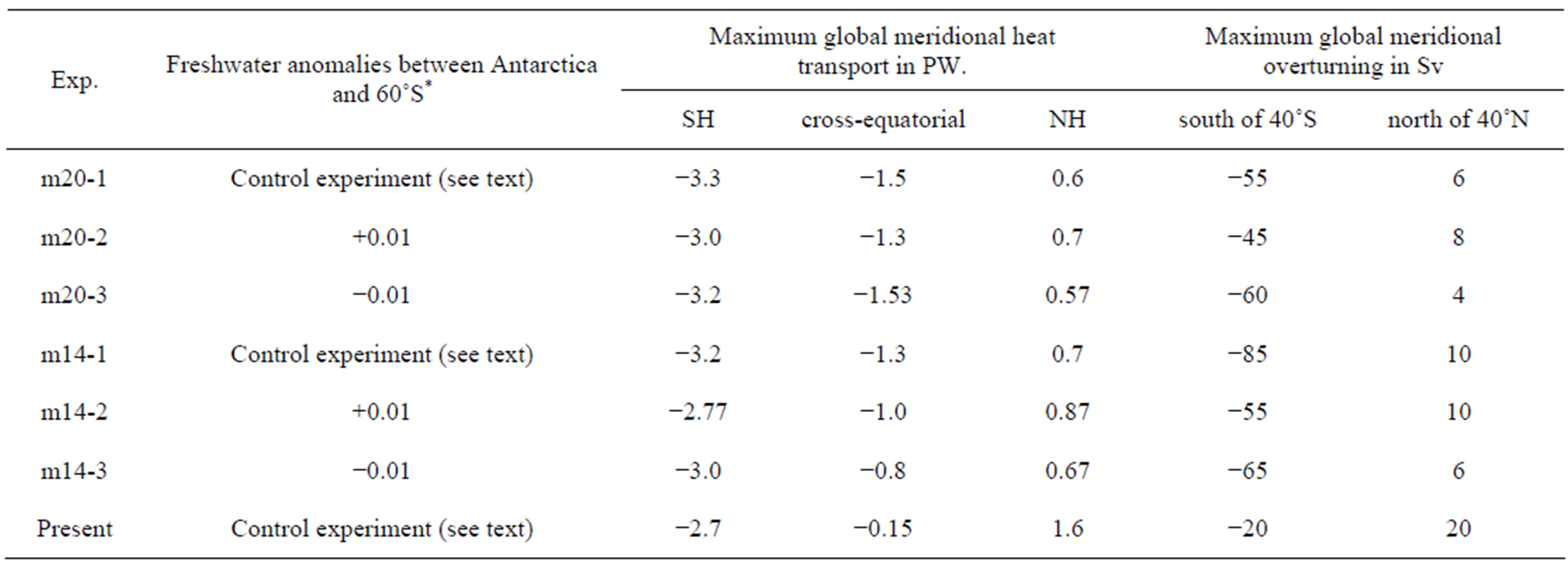
Table 1. Freshwater fluxes between the coast Antarctica and 60˚S. (*Added/removed water is redistributed over the entire sea surface to conserve water and salt balance in the World Ocean. Plus means added freshwater (hosing; fresher surface water), and minus means removal of freshwater (saltier surface water). The rates are in Sv; m20 stands for early Miocene (~20 Ma) and m14 for middle Miocene (~14 Ma)). The meridional heat transport is defined as a positive number if the transport is directed northward. The same applies for the meridional overturning.
on southern high-latitudinal oceanic freshwater changes leaving possible effects of the Tethys throughflow pit of the scope of our research.
Regarding the legitimacy of the offline coupling of model elements, we agree with von der Heydt and Dijkstra [56] that using offline coupled models may actually help in understanding and isolating the effect of certain forcings, e.g., due to the lack of direct feedback from the atmosphere.
Each of the two sets of experiments consists of a control run with undisturbed air-sea water exchanges, and the runs with locally increased or decreased freshwater fluxes tied to possible cryosphere melting or growing. The nature or dynamics of those melting/growing processes are beyond the scope of our study (e.g., changes in CO2 or albedo). We only presume, based on available estimates, that they were large enough to cause substantial disturbances of freshwater fluxes within the oceanice-atmosphere system.
Perturbing freshwater fluxes by adding or removing freshwater is conventionally referred to as “hosing” freshwater at the sea surface (e.g., Stouffer et al. [29]). In our experiments, freshwater is added (fresher surface water) or removed (saltier surface water) around Antarctica, i.e., sea surface salinity is changed with sea surface temperature remaining unaltered. Experiment setups and some key results are summarized in Table 1.
Both control ocean experiments start from an initially homogeneous ocean state with a temperature of 4˚C and a salinity of 34.25 psu (practical salinity unit) everywhere and continue for 10000 years of model time (Table 1, Exp. m20-1 and m14-1). The OGCM is forced using the output from the AGCM, which is being run for 20 years in the “slab ocean” mode. The resulting wind stress, temperature, and freshwater fluxes are averaged over the last 10 years of the AGCM simulations and converted into boundary conditions suitable for OGCM. The 20-year integration time and 10-year averaging period was proved to be sufficient for the AGCM to reach equilibrium (Dickens [34]). Each OGCM control experiment runs for 10,000 years and reaches a complete equilibrium (Seidov and Haupt [41]). It does not imply that the freshwater spike lasted 10,000 years; here it only means that after the startup of the spike (one could say that this would be the year 10,001), the ocean-atmosphere system reaches complete equilibrium including the deep ocean; the upper 1 km of water adjusts far quicker— within less than a hundred years.
The freshwater hosing experiments are referred to as Exps. m20-1 and m14-1. In these experiments the freshwater fluxes across the sea surface in a belt between Antarctica and the 60˚S parallel are perturbed to mimic relatively short-term episodes of melting or buildup of the Antarctic ice sheet.
Adding freshwater (hosing) in the model reflects ice melting (Table 1); freshwater removal is an equivalent of salinity rise due to brine rejection process or depositing frozen sea water in the Antarctic ice sheets. Addition or removal are of rather modest rate of only 0.01 Sv (1 Sv = 106 m3/s). The hosing experiments were started from the two control runs and continued for 500 years each. The results show the state of the ocean at the end of each simulation, i.e., after year 10,000 for the control experiments and year 10,500 for the hosing experiments.
The volume of freshwater added or being removed is fairly moderate. It amounts to approximately 1.58 e14 m3 over the period of 500 years. Langebroek et al. [17] estimate that a small ice sheet in the middle Miocene would have approximately a volume of 5 e15·m3 which would be equivalent of approximately 10 m layer of fresh water needed to build up such an ice sheet. Thus, our relatively small freshwater flux of 0.01 Sv corresponds to approximately 3% - 4% of the volume of a small ice sheet or a change of approximately 0.3 - 0.4 m in sea level. DeConto and Pollard [57] carried out ice sheet modeling experiments resulting in the Antarctic ice sheet growth of approximately 15 e15·m3 over a period of 30 kyr while Langebroek et al. [58] sensitivity experiments produce a change in ice volume of about 20 e15·m3 in 50 krs, which corresponds to 0.01 - 0.02 Sv.
3. RESULTS
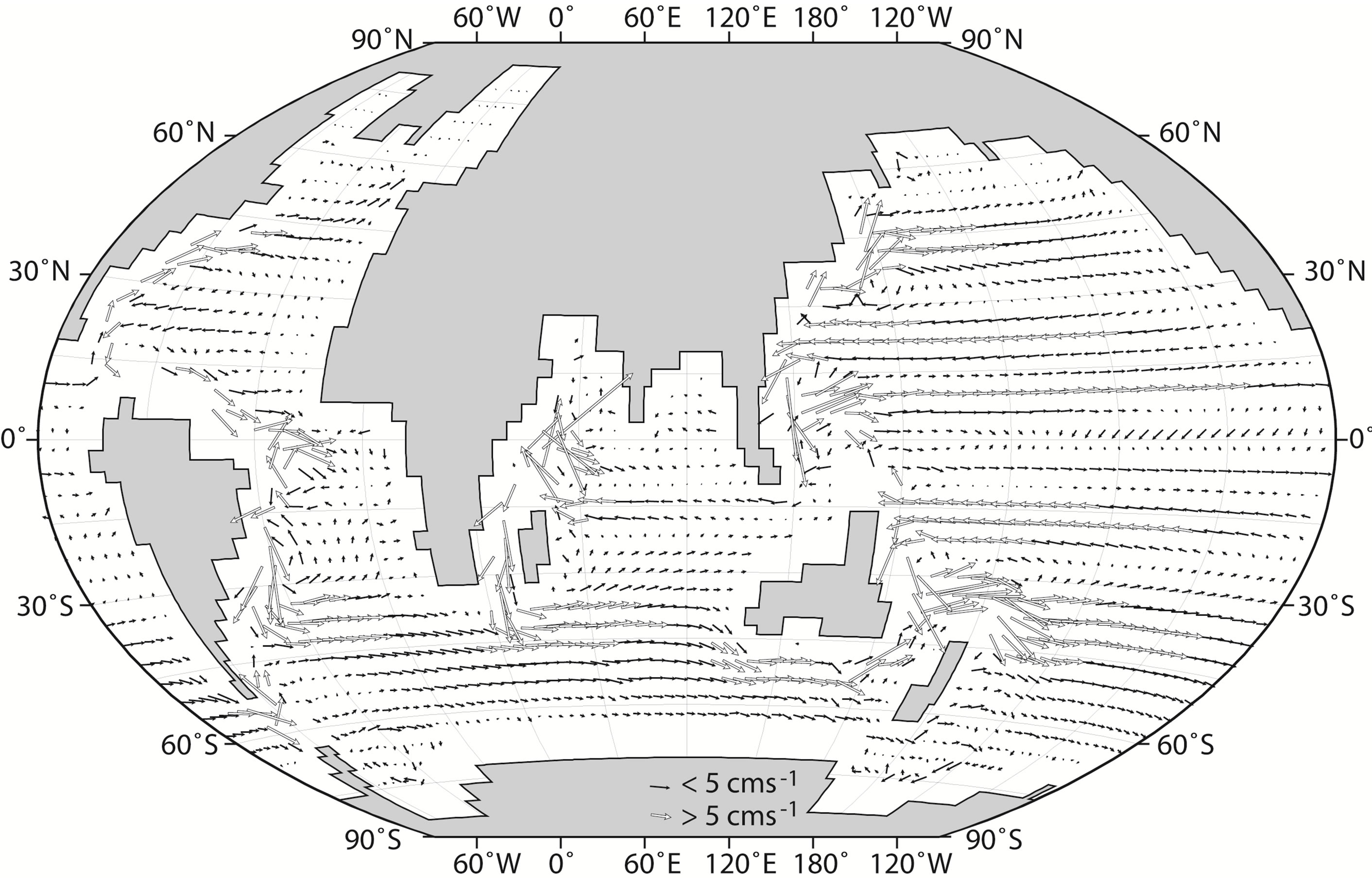
Figure 2 shows two patterns of ocean circulation at 75 m in experiments m20-1 and m14-1 (Table 1). Patterns of ocean circulation in the two control experiments are noticeably different except for an emerging North Atlantic Current and the onset of a proto-ACC which are clearly present in both runs. However, despite the fact that the Miocene land-sea geometry has much in common with the present-day geometry; a strong presentday-type Atlantic meridional overturning has not yet developed (Table 1). The North Atlantic Deepwater Formation in our computer runs increased from 20 to 14 Ma, which agrees with Woodruff and Savin [54].
Comparison of Exp. m20-2 and m14-2 to their respective control experiments (Exp. m20-1 and m14-1) reveals that the Miocene ocean is far more sensitive to freshening of the Southern Ocean than its present-day analogue (as, for example, in experiments by Stouffer et al. [29]). Adding freshwater around Antarctica leads to ~20% reduction of the southward cross-equatorial global heat transport in both Miocene cases if compared to the control experiments (Table 1). However, the heat transport maxima in both hemispheres are much stronger affected by freshwater hosing in the middle Miocene (compare Exps. m20-1 and m20-2 and Exps. m14-1 and m14-2, respectively).
 (a)
(a) (b)
(b)
Figure 2. Horizontal ocean velocities at 75 m depth: (a) Exp. m20-1 and (b) Exp. m14-1.
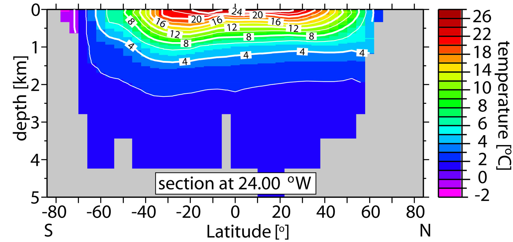
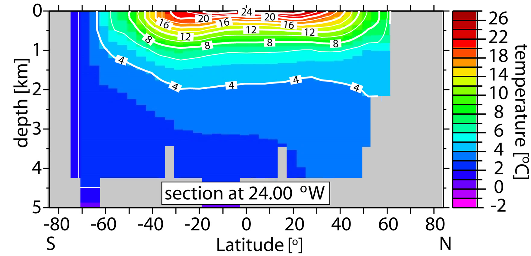
Figure 3 shows temperature sections along 24˚W and 168˚W, i.e., in the Atlantic and Pacific Ocean, respectively, at 20 Ma. Figure 4 depicts the same for 14 Ma. The upper panels show temperature in the control runs, whereas the middle and bottom panels show temperature differences relative to the control experiments.
The analysis of meridional overturning circulation (not shown) indicates that freshening of the sea surface causes much stronger reduction in deepwater formation south of 40˚S at 14 Ma than at 20 Ma. The increased northward oceanic heat transport and increased deepwater formation does lead to a slightly stronger pumping of warmer water into the deep ocean in the Northern Hemisphere (NH) at 20 Ma (Figures 3(c) and (d)). However, there is no significant increase in deepwater formation in the NH at 14 Ma (Table 1), contradicting a simple bipolar seesaw scheme. If the bi-polor scheme were valid, the significant drop of deepwater production in the Southern Hemisphere (SH) from –85 Sv to –55 Sv in the 14 Ma hosing experiment (Exp. m14-2, Table 1) would have led to noticeably stronger northbound overturning. Therefore, we argue that ocean-land geometry has the major control on deepwater formation in high latitudes.
The amplitude and duration of the freshwater impacts
 (a)
(a)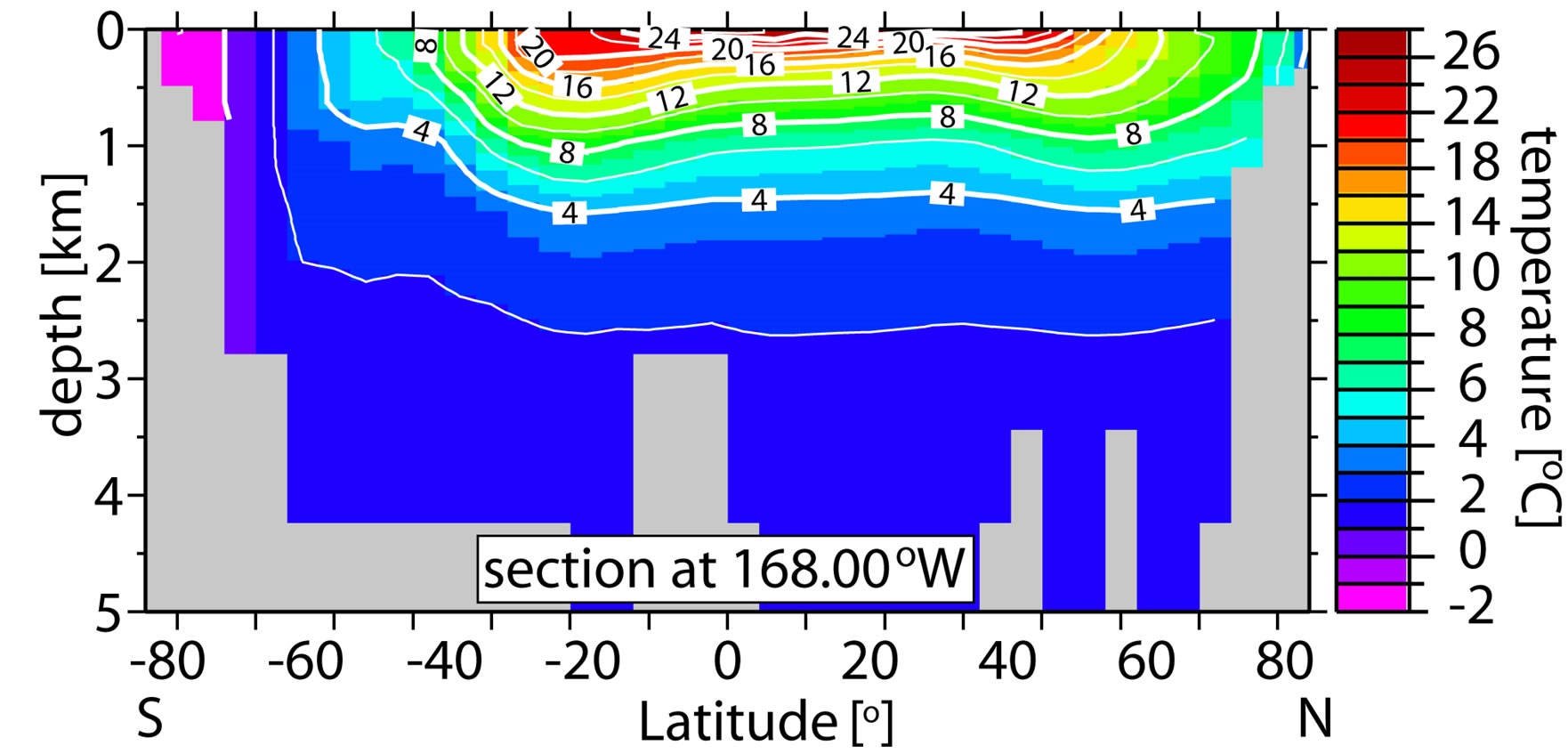 (b)
(b) (c)
(c)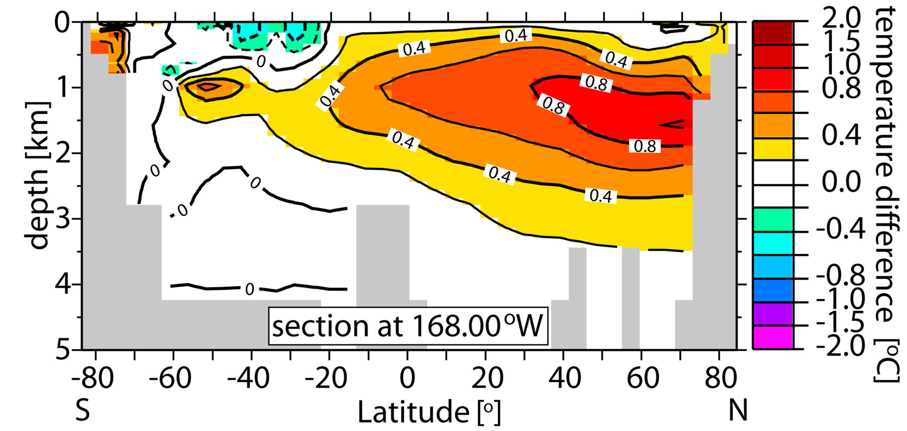 (d)
(d) (e)
(e)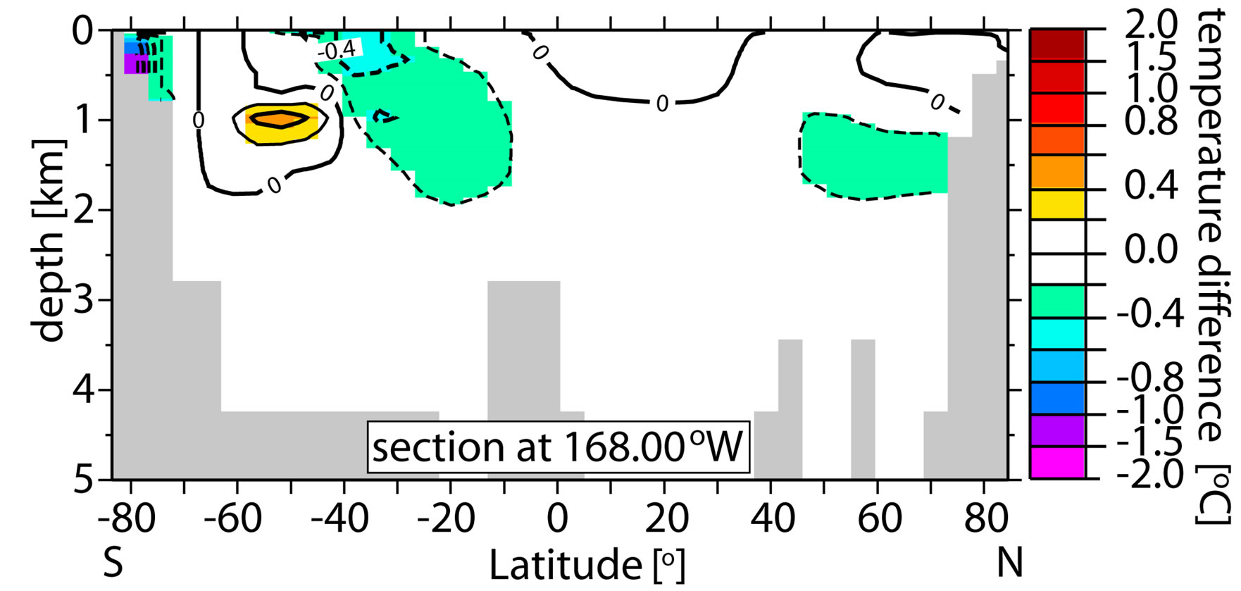 (f)
(f)
Figure 3. Temperature sections in the Atlantic (left column) and Pacific Oceans (right column) for 20 Ma: (a) and (b) Exp. m20-1; (c) and (d) Exp. m20-2 minus m20-1; (e) and (f) Exp. m20-3 minus m20-1.
are identical in both sets of experiments and the background atmospheric boundary conditions are very similar as well. Yet the response of the deep ocean to a southern freshening impact is noticeably different for 20 and 14 Ma. In sharp contrast to the 20 Ma simulation, the expected warming of the deep ocean did not happen in the 14 Ma experiment. Warming occurs mostly in the upper ocean in the NH and in the southern tropics. In fact, this warming of the upper ocean occurs coincidently with cooling of the deep ocean. It is not yet clear what might have caused such counter-intuitive behavior; we would anticipate rather a warming of the deep ocean due to reduced formation of proto Southern Ocean water.
Salinizing of proto Southern Ocean water around Antarctica increases the sea surface density during the early Miocene experiment m20-3. The consequences of such density increase in the south cause important changes of meridional transport in the northern North Atlantic. The meridional overturning north of 40˚N and the meridional overturning south of 40˚S decrease in transport. Decrease here means increase in magnitude; the overturning is negative in the southern hemisphere. That is, there are lower negative values of the northward transport south of 40S, meaning higher values of the southward transport. Those changes translate into more deepwater formation in the southern ocean and therefore higher southward heat transport. Consequently, the “heat piracy” (“stealing” heat from the opposite hemisphere (e.g., Seidov and Maslin [59]); the meridional heat transport is defined as a positive number if the transport is directed northward) decreases from −1.5 PW to −1.53 PW, i.e., the Southern Hemisphere gains additional heat (Table 1) (1 PW = 1015 W). Salinizing in the SH does not seem to have any sizable effect on temperature in the early Miocene simulation. This outcome supports the idea of lower SST, rather than higher sea surface salinity (SSS), being a primary control of the southern overturning. In contrast, freshening can hamper the overturning even if temperature remains close to freezing point. Meridional temperature sections in both the Atlantic and Pacific do not
 (a)
(a)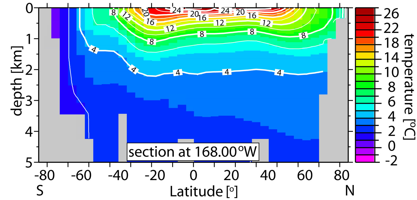 (b)
(b)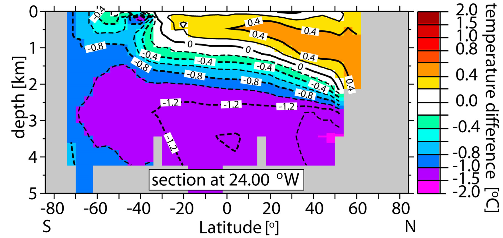 (c)
(c)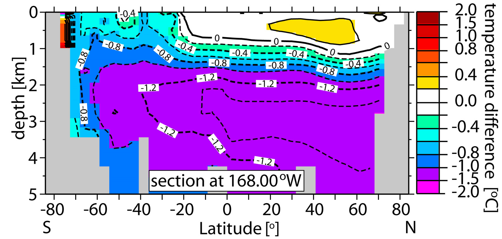 (d)
(d)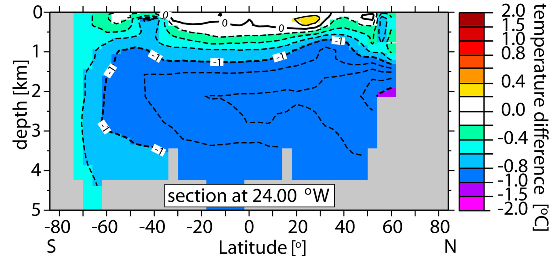 (e)
(e)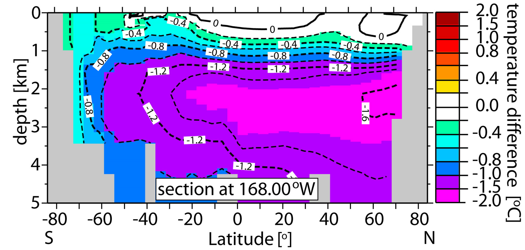 (f)
(f)
Figure 4. As in Figure 3 for 14 Ma. Temperature sections in the Atlantic (left column) and Pacific Oceans (right column): (a) and (b) Exp. m14-1; (c) and (d) Exp. m14-2 minus m14-1; (e) and (f) Exp. m14-3 minus m14-1.
change noticeably in the deep ocean (Figures 3(e) and (f)).
The middle Miocene experiment (Exp. m14-3) shows that surface salinizing in this run does indeed cause deep-ocean temperatures to cool by approximately 1 to 1.5˚C (Figures 4(e) and (f)). Counter-intuitively, the meridional overturning south of 40˚S drops from −85 Sv to −65 Sv and the oceanic cross-equatorial heat transport decreases from −1.3 PW to −0.8 PW, i.e., the Northern Hemisphere loses less heat. Usually it might be expected that freshening would reduce deepwater formation while a densification (caused both by cooling and salinizing) would increase the rate; we emphasize that we do not change any parameter other than freshwater fluxes nor do we have an atmospheric feedback. Thus we have a pure effect of just one element—the change in SSS (von der Heydt and Dijkstra [56]).
4. DISCUSSION AND CONCLUSIONS
We hope that our results are shedding some additional light on whether ocean changes might have accompanied the fluctuation of the sea ice extend of the Antarctic Ice Sheet in the Miocene. The numerical experiments imply higher sensitivity of the Miocene ocean circulation to freshwater hosing in the proto Southern Ocean than of the present-day climate. One possible explanation is that the opening of the Central American Isthmus could be responsible for a stronger than present-day sensitivity of the ocean thermohaline circulation to small freshwater disturbances in the Southern Ocean around Antarctica. However, we cannot rule out that other effects, e.g., orbital parameters, a more narrow Drake passage, a further southward drift of Australia, New Zealand, and Indonesia and thus a opening of the Australo-Antarctic seaway, as well as a number of other perhaps less important factors that collectively might have also been responsible for the increased sensibility. Moreover, we cannot rule out that other changes, even those far away from the Southern Ocean, such as subsidence of the Iceland Faeroe Ridge allowing the Norwegian Overflow Water into the North Atlantic, can be held responsible for increased sensitivity. In order to test each element of the impact factors, numerous experiments for each case would be necessary, which is not currently feasible.
The 20 and 14 Ma experiment configurations differ basically only in ocean-land geometry, yet the overall ocean’s response to exactly the same freshwater impacts is strikingly different. Thus it is a plausible assumption that the geometry of the proto-ACC is responsible for these differences.
In conclusion, we argue that relatively small and geologically short-lived changes in freshwater balance in the Southern Ocean could be responsible, at least partially, for two prominent disruptions (20 and 14 Ma) of the dynamic Miocene’s general cooling trend. Finally, we also argue that the widely accepted bi-polar scheme of the ocean circulation changes may need to be revisited to include a strong geometry control for paleoclimates with noticeably different sea-ice geometry.
5. ACKNOWLEDGEMENTS
This study was partly supported by NSF (NSF projects # 0224605 and ATM 00-00545). The views, opinions, and findings contained in this report are those of the authors and should not be construed as an official NOAA or U.S. Government position, policy, or decision. The authors express their gratitude to two anonymous reviewers for their comments that helped to improve the manuscript.
REFERENCES
- Crowley, T.J. and North, G.R. (1991) Paleoclimatology. Oxford University Press, New York.
- Thomas, E. (2008) Descent into the icehouse. Geology, 36, 191-192. doi:10.1130/focus022008.1
- Pagani, M., Zachos, J.C., Freeman, K.H., Tipple, B. and Bohaty, S. (2005) Marked decline in atmospheric carbon dioxide concentrations during the Paleogene. Science, 309, 600-603. doi:10.1126/science.1110063
- Shellito, C.J., Sloan, L.C. and Huber, M. (2003) Climate model sensitivity to atmospheric CO2 levels in the EarlyMiddle Paleogene. Palaeogeography, Palaeoclimatology, Palaeoecology, 193, 113-123. doi:10.1016/S0031-0182(02)00718-6
- Zachos, J.C., Dickens, G.R. and Zeebe, R.E. (2008) An early Cenozoic perspective on greenhouse warming and carbon-cycle dynamics. Nature, 451, 279-283. doi:10.1038/nature06588
- Barron, E.J. and Peterson, W.H. (1991) The Cenozoic ocean circulation based on ocean general circulation model results. Palaeogeography, Palaeoclimatology, Palaeoecology, 83, 1-28. doi:10.1016/0031-0182(91)90073-Z
- Bice, K.L., Scotese, C.R., Seidov, D. and Barron, E.J. (2000) Quantifying the role of geographic change in Cenozoic ocean heat transport using uncoupled atmosphere and ocean models. Palaeogeography, Palaeoclimatology, Palaeoecology, 161, 295-310. doi:10.1016/S0031-0182(00)00072-9
- Seidov, D.G. (1986) Auto-oscillations in the system largescale circulation and synoptic ocean eddies. Isvestiya, Atmospheric and Oceanic Physics, 22, 679-685.
- Pekar, S.F. (2008) Climate change: When did the icehouse cometh? Nature, 455, 602-603. doi:10.1038/455602a
- Bell, R.E., Luydendy, B.P. and Wilson, T.J. (2008) Antarctica: A keystone in a changing world. EOS, 89, 4. doi:10.1029/2008EO010005
- Pekar, S.F. and Deconto, R.M. (2006) High-resolution ice-volume estimates for the early Miocene: Evidence for a dynamic ice sheet in Antarctica. Palaeogeography, Palaeoclimatology, Palaeoecology, 231, 101-109. doi:10.1016/j.palaeo.2005.07.027
- Abreu, V.S. and Anderson, J.B. (1998) Glacial eustacy during the Cenozoic: Sequence stratigraphic implications. American Association Petroleum Geologists Bulletin, 82, 1385-1400.
- Zachos, J., Pagani, M., Sloan, L., Thomas, E. and Billups, K. (2001) Trends, rhythms, and aberrations in global climate 65 Ma to present. Science, 292, 686-693. doi:10.1126/science.1059412
- Lear, C.H., Mawbey, E.M. and Rosenthal, Y. (2010) Cenozoic benthic foraminiferal Mg/Ca and Li/Ca records: Toward unlocking temperatures and saturation states. Paleoceanography, 25, 1-11. doi:10.1029/2009PA001880
- Boehme, M. (2003) The miocene climatic optimum: Evidence from ectothermic vertebrates of central Europe. Palaeogeography, Palaeoclimatology, Palaeoecology, 195, 389-401. doi:10.1016/S0031-0182(03)00367-5
- Holbourn, A., Kuhnt, W., Schulz, M. and Erlenkeuser, H. (2005) Impacts of orbital forcing and atmospheric carbon dioxide on Miocene ice-sheet expansion. Nature, 438, 483-487. doi:10.1038/nature04123
- Langebroek, P.M., Paul, A. and Schulz, M. (2010) Simulating the sea level imprint on marine oxygen isotope records during the middle Miocene using an ice sheet-climate model. Paleoceanography, 25, 1-12. doi:10.1029/2008PA001704
- Pagani, M., Caldeira, K., Berner, R. and Beerling, D.J. (2009) The role of terrestrial plants in limiting atmospheric CO2 decline over the past 24 million years. Nature, 460, 85-88. doi:10.1038/nature08133
- Deconto, R.M., Pollard, D., Wilson, P.A., Palike, H., Lear, C.H. and Pagani, M. (2008) Thresholds for cenozoic bipolar glaciation. Nature, 455, 652-657. doi:10.1038/nature07337
- Kump, L.R. (2009) Tipping pointedly colder. Science, 323, 1175-1176. doi:10.1126/science.1170613
- Bice, K.L. and Marotzke, J. (2001) Numerical evidence against reversed thermohaline circulation in the warm Paleocene/Eocene ocean. Journal of Geophysical Research, 106, 11529-511542. doi:10.1029/2000JC000561
- Haupt, B.J. and Seidov, D. (2001) Warm deep-water ocean conveyor during the Cretaceous time. Geology, 29, 295-298. doi:10.1130/0091-7613(2001)029<0295:WDWOCD>2.0.CO;2
- Haupt, B.J. and Seidov, D. (2007) Strengths and weaknesses of the global ocean conveyor: Inter-basin freshwater disparities as the major control. Progress in Oceanography, 73, 358-369. doi:10.1016/j.pocean.2006.12.004
- Seidov, D., Barron, E.J. and Haupt, B.J. (2001) Meltwater and the global ocean conveyor: Northern versus southern connections. Global and Planetary Change, 30, 253-266. doi:10.1016/S0921-8181(00)00087-4
- Seidov, D., Sarnthein, M., Stattegger, K., Prien, R. and Weinelt, M. (1996) North Atlantic ocean circulation during the Last Glacial Maximum and subsequent meltwater event: A numerical model. Journal of Geophysical Research, 101, 16305-16332. doi:10.1029/96JC01079
- Rahmstorf, S. (1995) Bifurcations of the Atlantic thermohaline circulation in response to changes in the hydrological cycle. Nature, 378, 145-149. doi:10.1038/378145a0
- Schmittner, A., Meissner, K.J., Eby, M. and Weaver, A.J. (2002) Forcing of deep ocean circulation in simulation of the Last Glacial Maximum. Paleoceanography, 17, 15.
- Stocker, T.F., Wright, D.G. and Broecker, W.S. (1992) The influence of high-latitude surface forcing on the global thermohaline circulation. Paleoceanography, 7, 529-541. doi:10.1029/92PA01695
- Stouffer, R.J., Seidov, D. and Haupt, B.J. (2007) Climate response to external sources of freshwater: North Atlantic versus the Southern ocean. Journal of Climate, 20, 436- 448. doi:10.1175/JCLI4015.1
- Weaver, A.J., Saenko, O.A., Clark, P.U. and Mitrovica, J.X. (2003) Meltwater pulse 1A from Antarctica as a trigger of the Bølling-Allerød warm interval. Science, 299, 1709-1713. doi:10.1126/science.1081002
- Cox, M. and Bryan, K. (1984) A numerical model of the ventilated thermocline. Journal of Physical Oceanography, 14, 674-687. doi:10.1175/1520-0485(1984)014<0674:ANMOTV>2.0.CO;2
- Butzin, M., Lohmann, G. and Bickert, T. (2011) Miocene ocean circulation inferred from marine carbon cycle modeling combined with benthic isotope records. Paleoceanography, 26, 1-19. doi:10.1029/2009PA001901
- Herold, N., Mueller, R.D. and Seton, M. (2010) Comparing early to middle Miocene terrestrial climate simulations with geological data. Geosphere, 6, 952-961. doi:10.1130/GES00544.1
- Dickens, J.M. (2004) Ocean-atmosphere feedback in climate simulations using off-line modules of a coupled oceanatmosphere model. Master’s Thesis, Pennsylvania State University, University Park.
- Barron, E.J. and Moore, G.T. (1994) Climate model applications in paleoenvironmental analysis. Geological Society Publishing, Tulsa.
- Vertenstein, M. and Kluzek, E.B. (1999) User’s guide to LSM1.1. National Center for Atmospheric Research, Boulder.
- Kluzek, E.B., Olson, J., Rosinski, J.M., Truesdale, J.E. and Vertenstein, M. (1999) User’s guide to NCAR CCM 3.6, National Center for Atmospheric Research, Boulder.
- Pacanowski, R.C. (1996) User’s guide and reference manual, GFDL Ocean Technical Report, Geophysical Fluid Dynamics Laboratory, Princeton.
- Herrmann, A.D. (2003) Late Ordovician ocean-climate system and paleobiogeography. Dissertation, Pennsylvania State University, University Park.
- Herrmann, A.D., Haupt, B.J., Patzkowsky, M.E., Seidov, D. and Slingerland, R.L. (2004) Response of Late Ordovician paleoceanography to changes in sea level, continental drift, and atmospheric pCO2: Potential causes for long-term cooling and glaciation. Palaeogeography, Palaeoclimatology, Palaeoecology, 210, 385-401. doi:10.1016/j.palaeo.2004.02.034
- Seidov, D. and Haupt, B.J. (1997) Global ocean thermohaline conveyor at present and in the late Quaternary. Geophysical Research Letters, 24, 2817-2820. doi:10.1029/97GL02913
- Seidov, D. and Haupt, B.J. (2003) On sensitivity of ocean circulation to sea surface salinity. Global and Planetary Change, 36, 99-116. doi:10.1016/S0921-8181(02)00177-7
- Seidov, D. and Haupt, B.J. (2003) Freshwater teleconnections and ocean thermohaline circulation. Geophysical Research Letters, 30, 1-4. doi:10.1029/2002GL016564
- Seidov, D. and Haupt, B.J. (2005) How to run a minimalist's global ocean conveyor. Geophysical Research Letters, 32, 1-4. doi:10.1029/2005GL022559
- Eldridge, J., Walsh, D. and Scotese, C.R. (2002) PALEOMAP Paleogeographic Atlas. www.scotese.com
- Scotese, C.R. (1997) Paleogeographic Atlas, PALEOMAP Progress Report 90-0497. University of Texas at Arlington, Arlington.
- Scotese, C.R., Ross, M.I. and Schettino, A. (1998) Plate tectonic reconstruction and animation. EOS, 79, 334.
- Toggweiler, J.R. and Bjornsson, H. (2000) Drake Passage and palaeoclimate. Journal of Quarternary Science, 15, 319-328. doi:10.1002/1099-1417(200005)15:4<319::AID-JQS545>3.0.CO;2-C
- Maier-Reimer, E., Mikolajewicz, U. and Crowley, T. (1990) Ocean general circulation model sensitivity experiment with an open central American isthmus. Paleoceanography, 5, 349-366. doi:10.1029/PA005i003p00349
- Tong, J.A., You, Y., Müller, R.D. and Seton, M. (2009) Climate model sensitivity to atmospheric CO2 concentrations for the middle Miocene. Global and Planetary Change, 67, 129-140. doi:10.1016/j.gloplacha.2009.02.001
- Von Der Heydt, A. and Dijkstra, H.A. (2005) Flow reorganizations in the Panama Seaway: A cause for the demise of Miocene corals? Geophysical Research Letters, 32, 1-4. doi:10.1029/2004GL020990
- Jovane, L., Coccioni, R., Marsili, A. and Acton, G. (2009) The late Eocene greenhouse-icehouse transition: Observations from the Massignano global stratotype section and point (GSSP). In: Koeberl, C. and Montanari, A., Eds., The Late Eocene Earth: Hothouse, Icehouse, and Impacts, Geological Society of America, Boulder, 149-168. doi:10.1130/2009.2452(10)
- Roegl, F. (1999) Mediterranean and paratethys. Facts and hypotheses of an oligoncene to miocene paleogeography (short overview). Geologica Carpathica, 50, 330-349.
- Woodruff, F. and Savin, S.M. (1989) Miocene deepwater oceanography. Paleoceanography, 4, 87-140. doi:10.1029/PA004i001p00087
- Herold, N., Seton, M., Mueller, R.D., You, Y. and Huber, M. (2008) Middle Miocene tectonic boundary conditions for use in climate models. Palaeogeography, Palaeoclimatology, Palaeoecology, 9, 1-10.
- Von Der Heydt, A. and Dijkstra, H.A. (2008) The effect of gateways on ocean circulation patterns in the Cenozoic. Global and Planetary Change, 62, 132-146. doi:10.1016/j.gloplacha.2007.11.006
- Deconto, R.M. and Pollard, D. (2003) A coupled climate-ice sheet modeling approach to the Early Cenozoic history of the Antarctic ice sheet. Palaeogeography, Palaeoclimatology, Palaeoecology, 198, 39-52. doi:10.1016/S0031-0182(03)00393-6
- Langebroek, P.M., Paul, A. and Schulz, M. (2009) Antarctic ice-sheet response to atmospheric nd insolation in the Middle Miocene. Climate of the Past, 5, 633-646. doi:10.5194/cp-5-633-2009
- Seidov, D. and Maslin, M. (2001) Atlantic Ocean heat piracy and the bi-polar climate sea-saw during Heinrich and Dansgaard-Oeschger events. Journal of Quaternary Science, 16, 321-328. doi:10.1002/jqs.595