Engineering
Vol.08 No.04(2016), Article ID:65833,23 pages
10.4236/eng.2016.84016
Simple Adaptive Delta Operator Aircraft Flight Control for Accommodation of Loss of Control Effectiveness
Alfredo Cano, Kenneth Sobel*
Department of Electrical Engineering, The City College of New York, New York, NY, USA

Copyright © 2016 by authors and Scientific Research Publishing Inc.
This work is licensed under the Creative Commons Attribution International License (CC BY).
http://creativecommons.org/licenses/by/4.0/


Received 10 February 2016; accepted 20 April 2016; published 25 April 2016
ABSTRACT
A new proof for stability of delta operator simple adaptive control is presented in terms of a set of Linear Matrix Inequalities (LMIs). The paper shows how to design a feedforward gain to satisfy the LMIs over a polytope of loss of control effectiveness failures. The MATLAB Robust Control Toolbox is used to find the feedforward gain with the smallest norm that satisfies the LMIs. Examples are presented of the F/A-18 aircraft and the Innovative Control Effectors (ICE) tailless aircraft that show the design of a feedforward gain for a loss of control effectiveness in any one control effector. The designs use a fixed eigenstructure assignment controller for an inner loop augmented with the simple adaptive controller. Simulations of both aircraft include simultaneous loss of control effectiveness failure and lateral wind gust. Simulation results for the F/A-18 aircraft show that the adaptive controller achieves almost perfect tracking whereas the nonadaptive controller cannot achieve a coordinated turn when an aileron failure occurs. The ICE tailless aircraft uses sideslip, washed-out stability axis yaw rate, and stability axis roll rate feedback for both the inner loop eigenstructure assignment controller and the simple adaptive controller. However, the adaptive controller also uses bank angle feedback. Simulation results for the ICE tailless aircraft show that the adaptive controller achieves almost perfect tracking whereas the nonadaptive controller diverges when an all moving tip failure occurs.
Keywords:
Simple Adaptive Control, Delta Domain, Parallel Feedforward, Aircraft Control Failure

1. Introduction
Aircraft flight control systems are designed with extensive redundancy to ensure a low probability of failure. During recent years, however, several aircraft have experienced major control system failures. These have caused an increased interest in fault tolerant flight control systems. The objective of a fault tolerant flight control system is to control and safely land the aircraft in case of severely damaged or inoperable control surfaces. One of the approaches to fault tolerant control is active control. An active fault tolerant control system has to either reconfigure or adapt the controller in response to the failure. Typical design methods include multiple model, switching, and tuning designs; adaptive designs; and fault detection and diagnosis designs. Adaptive failure accommodation designs have simpler control structures and do not rely on knowledge of the actuator failures. Direct adaptive designs use the system response error to achieve desired performance.
Early results similar to Simple Adaptive Control (SAC) were obtained by Fradkov [1] in Russia as early as 1974-1976. Independently, Sobel, Kaufman, and Mabius [2] [3] proposed a related approach in the USA in the late 1970s. This result was extended and given the name simple adaptive control by Barkana and Kaufman [4] [5] who inserted a feedforward compensator around the plant so that the augmented system was Almost Strictly Positive Real (ASPR). Kaufman, Barkana, and Sobel [6] summarized stability results which showed that all signals in the adaptive system were bounded and that the augmented error was asymptotically vanishing if the augmented plant was ASPR. Other results in the design of parallel feedforward compensators which realized an ASPR augmented system were developed by Mizumoto, Fukui, Yamanaka, and Shah [7] using the Fictitious Reference Iterative Tuning (FRIT) method.
Many authors have applied SAC to aerospace problems. For example, Mooij [8] has applied SAC to an Apollo shaped re-entry vehicle; Rusnak, Weiss, and Barkana [9] have applied SAC to a missile autopilot; and Luzi, Peaucelle, Biannic, Pittet, and Mignot [10] add a gain barrier function to SAC with application to attitude control of a satellite. Ulrich and Sasiadek [11] have extended SAC by using a decentralized adaptation law with application to a rigid joint manipulator.
Belkharraz and Sobel [12] extended the work of Kaufman, Barkana, and Sobel [6] to include loss of control effectiveness failures. The percentage loss of control effectiveness is unknown and may be arbitrarily close to a complete loss subject to the satisfaction of the sufficient conditions for stability. A state space approach was introduced for computing the feedforward compensator which guarantees that the augmented plant is ASPR by using the MATLAB®LMI and Optimization toolboxes. Belkharraz and Sobel [13] extended this work to include bounded input disturbances. It was proven that all signals were bounded for loss of control effectiveness failures during a bounded input disturbance.
Barkana [14] and Ben-Yamin, Yaesh and Shaked [15] extended simple adaptive control to discrete time systems using a shift operator model. A disadvantage of the shift operator model is that the eigenvalues all approach unity as the sampling period goes to zero. Belkharraz and Sobel [16] extended simple adaptive control to Middleton and Goodwin’s [17] delta domain model. This model is valid for both continuous time and sampled data operation of the plant. An important property of the delta domain model is that the discrete time eigenvalues approach the continuous time eigenvalues as the sampling period approaches zero. Belkharraz and Sobel [16] proved that all signals were bounded for loss of control effectiveness failures during a bounded disturbance. The simple adaptive control algorithm was applied to a three input model of the linearized lateral dynamics of the F/A-18 aircraft. However, [16] used the feedforward of [13] that was designed for the continuous time model of the F/A-18 aircraft. The extension of the feedforward design method [12] to delta operator systems was left as an open question.
In this paper, a new proof for stability of delta operator simple adaptive control is presented in terms of a set of Linear Matrix Inequalities (LMIs). The paper shows how to design a feedforward gain to satisfy the LMIs over a polytope of loss of control effectiveness failures. The results in this paper are an explicit function of the sampling period Δ. The MATLAB Robust Control Toolbox [18] is used to find the feedforward gain with smallest norm that satisfies the LMIs. Barkana, Rusnak, and Weiss [19] have shown that a constant parallel feedforward gain D can be implemented as part of the adaptive controller. Therefore, nothing is added in parallel with the plant in the implementation of our adaptive controller. Examples are presented of the F/A-18 aircraft [12] and the Innovative Control Effectors (ICE) tailless aircraft [20] that show the design of a feedforward gain for a loss of control effectiveness in any one control effector. Simulations of both aircraft include simultaneous loss of control effectiveness failure and lateral wind gust.
An example is presented of the F/A-18 aircraft [12] that shows the design of a feedforward gain for a loss of control effectiveness in any one control effector of either 92% trailing edge flap, 99% aileron, or 80% rudder. The design uses a fixed eigenstructure assignment controller for an inner loop augmented with the simple adaptive controller. Both loops use sideslip, washed-out yaw rate, and roll rate feedback sampled at 200 Hz. Simulation results show that the adaptive controller achieves almost perfect tracking whereas the nonadaptive controller cannot achieve a coordinated turn when an aileron failure occurs. A second example is presented of the ICE tailless aircraft [20] that shows the design of a feedforward gain for a loss of control effectiveness in any one control effector of either 50% elevon, 50% all moving tips, or 50% yaw thrust vectoring. Here both the inner loop eigenstructure assignment controller and the adaptive controller use sideslip, washed-out stability axis yaw rate, and stability axis roll rate feedback. However, the adaptive controller also uses bank angle feedback. Both loops use a sampling rate of 1 kHz. Simulation results show the adaptive controller achieves almost perfect tracking whereas the nonadaptive controller diverges when an all moving tip failure occurs.
A preliminary version of this paper [21] was presented at the AIAA Guidance, Navigation and Control Conference. This revised version includes 1) an extended explanation of the feedforward gain design method, 2) an extended discussion of almost strictly positive real and its relationship to minimum phase for delta operator systems, 3) the addition of a lateral wind gust to the ICE aircraft example, and 4) new time responses that are consistent for both examples with a control effectiveness failure at 5 sec and a lateral wind gust at 10 sec with a duration of 10 sec. The addition of a lateral wind gust to the ICE aircraft resulted in a more difficult problem. This problem was solved with the novel idea of adding bank angle feedback to the adaptive controller, but not the inner loop eigenstructure assignment controller, in order to achieve excellent tracking during a simultaneous loss of control effectiveness failure and lateral wind gust.
2. Problem Statement
Let ,
,  , with
  finite and
 , be the time intervals on which the control surface failure pattern is fixed. That is, control surfaces only fail at time
 ,
, . Then, the plant on the interval
 ,
,  is described by
 (1)
(1)
where  is the plant state vector,
  is the control input,
  is a bounded input disturbance,
  is the plant output, and matrices
  are of the appropriate dimensions.
 (2)
(2)

Here the failure times are ; which control surfaces fail at
 ,
,  is unknown; the amount of the loss of effectiveness at
  given by
 , where
  is unknown. Furthermore, once a control surface fails it may fail again later with a different amount of loss of effectiveness.
The unified state space model proposed by Middleton and Goodwin [17] is valid for both the discrete and continuous time cases simultaneously. This unified model, which is assumed to be a minimal realization, is described by [21] :
 (3)
(3)
The plant in Equation (3) is augmented with a fixed feedforward gain matrix D and becomes
 (4)
(4)
so that  is the output to be controlled and where D is square and nonsingular. We remark that in augmenting the plant Equation (3) to obtain Equation (4) we are not physically modifying the system, instead we are just defining a metasystem that will allow us to use the simple adaptive control SAC methodology.
The control objective is to design an adaptive control signal  such that all signals in the closed loop system are bounded and the augmented plant output
  tracks the output of a reference model given by [21] :
 (5)
(5)
 (6)
(6)
We remark that the order of the plant may be much greater than the order of the reference model. That is, 
3. The General Tracking Problem
We summarize the general tracking problem for a known plant. These results have appeared in Kaufman, Barkana, and Sobel [6] and Barkana [5] . Let the input command  be the output of an unknown command generating systems of the form
 (7)
(7)
 (8)
(8)
Define the ideal trajectories , such that, if the augmented plant could reach and move along them, its output would perfectly track the output of the reference model. That is, the ideal trajectories are targets that the augmented plant tries to reach or at least be close to, in order to have bounded tracking errors. Mathematically,
 (9)
(9)
where the ideal trajectories are defined as
 (10)
(10)
and the ideal control signal is defined as
 (11)
(11)
Substituting  from Equation (10) into Equation (9), and using
  from Equation (8), gives a condition for the existence of the ideal target trajectories:
 (12)
(12)
or
 (13)
(13)
Since the number  of equations is smaller than the number
  of variables, the solutions for
  and
and  in Equation (13) are guaranteed. This implies the existence of some bounded trajectories in the
  space that the plant needs to attain perfect tracking. To see this, define
 and
and . Then substituting Equation (11) into the ideal augmented plant given by
 (14)
(14)
we obtain
 (15)
(15)
Therefore, the ideal control in Equation (11) and the ideal augmented plant in Equation (14) allow for perfect tracking. We now establish a necessary condition for perfect tracking in the following lemma.
Lemma 1: Perfect tracking is possible only if the augmented plant is ASPR and .
.
Proof: We can rewrite  as
as . Then after solving for
  and substituting into the augmented plant in Equation (4) with
  we obtain
 (16)
(16)
Thus, since the reference model is stable, we only require that  be stable, which is only true when the augmented plant given by
  is ASPR ( [6] , pp. 50-51).
In general, when the augmented plant does not satisfy the perfect tracking conditions due to a non-zero input disturbance , we look for a controller such as that proposed by Ben-Yamin, Yaesh, and Shaked [15] :
 (17)
(17)
with


where  is the error between the reference model output and the augmented plant output,
  ,
,  , and
, and  are stabilizing and bounded gains (since the reference model is stable and
  is bounded) and where
  is an auxiliary input signal. The control in Equation (17), however, requires calculations of
  and
and  and also explicit knowledge of the system dynamics. As an alternative, the direct adaptive control algorithm known as Simple Adaptive Control (SAC) is used to calculate the gains which enable the plant to get bounded tracking errors. Note that SAC only requires that the plant outputs be available for measurement.
4. Adaptive Control
Algorithm
The unified form of the adaptive algorithm is as follows

The adaptive gains are concatenated into matrix  defined as

The concatenated gain  is defined as the sum of a proportional gain
  and an integral gain
 , each of which is adapted as follows
 (18)
(18)
 (19)
(19)
 (20)
(20)
 (21)
(21)
 (22)
(22)
where
 (23)
(23)
and T and  are time invariant weighting matrices. The
  term in Equation (20) was originally proposed by Ioannou and Kokotovic [22] and it is used to avoid divergence of the integral gains in the presence of bounded disturbances.
5. Almost Strictly Positive Real and Minimum-Phase Concepts
The following development shows sufficient conditions for a system to be ASPR in the delta domain.
Lemma 2: The unified system described by the minimal realization in Equation (4), with , is SPR if and only if there exists a positive-definite symmetric matrix P that satisfies the following LMI
 (24)
(24)
Proof: The result follows trivially from Proposition 4 in Collins, Haddad, Chellaboina, and Song [23] and the observation that as , Equation (24) approaches the continuous time result given by Lemma 4 in Kottenstette and Antsaklis [24] .
Note that the SPR property for the unified model requires not only  (i.e. positive-definite D), as
in the continuous time result, but also that  for a positive-definite symmetric matrix P
that satisfies the LMI in Equation (24). Furthermore, the SPR property implies the unified model is asymptotically stable.
Since most systems are not inherently SPR, consider the stabilizing constant output feedback gain  in the control signal given by
 (25)
(25)
where  is an auxiliary input command to the closed loop. Substituting
  from Equation (4) into Equation (25) yields the following algebraic loop

or

Assuming that  exists, we obtain that

Now we make the following definition
 (26)
(26)
and note that . Thus the algebraic loop becomes
 (27)
(27)
Substituting Equation (27) into Equation (4), with , we obtain
 (28)
(28)
Letting ,
,  ,
,  and
and  we obtain the closed loop system
 (29)
(29)
Using Lemma 1 we have that Equation (29) is SPR (or Equation (4) is ASPR) if and only if there exists a positive-definite symmetric matrix P such that
 (30)
(30)
Now we derive necessary conditions for the unified system to be minimum-phase (MP). The zero dynamics are obtained from  of Equation (4) and are given by
 , which yields
 (31)
(31)
Substituting Equation (31) into the first equation of Equation (4), with , gives the zero-dynamics equation
 (32)
(32)
where . If the unified system in Equation (4) is MP then
  must be asymptotically stable. That is, Equation (4) is MP if there exist a positive-definite symmetric matrix P such that
 (33)
(33)
or, equivalently, all the eigenvalues of  must reside inside the circle of radius
  centered at
  in the complex plane. We are now in a position to state and prove the following lemma.
Lemma 3: If the unified system in Equation (4), with D nonsingular and , is MP, then it is ASPR.
Proof: Assume that the unified model in Equation (4) is MP and D is nonsingular. We want to show that there exists a stabilizing, positive-definite symmetric gain  sufficiently large that leads to a closed loop system that is SPR. To this end, consider the control signal of Equation (25) that leads to a closed loop system in Equation (28), which, using Equation (26), can be rewritten as
 (34)
(34)
Let  and
and  to obtain
 (35)
(35)
where  and
and . Applying the left-hand side of
Lemma 1 to Equation (35), and assuming a positive-definite symmetric matrix P, we have that
 (36)
(36)
where


Showing that L < 0 would imply that Equation (35) is SPR and, by noting that ,
,
that Equation (34) is also SPR or, equivalently, that Equation (4) is ASPR, as desired. Therefore we must show that for  sufficiently large,
 . To this end we use Schur’s complement lemma and note that
  is equivalent to
  and
and  ( [25] , p. 38).
First note that  follows from the assumption that Equation (4) is MP, since the zeros of the closed loop system with a constant output feedback gain
  are identical to the zeros of the open loop system [26] .
Next we show that . Consider
  in
in  and note that, since D is nonsingular and
 ,
,  is the only positive-definite term in
 . However, while
  and
and 
is nondefinite, these two terms are bounded and hence we can establish that, for a sufficiently large positive-defi-nite gain , the following inequality can be satisfied

Thus we will have , which is a necessary condition for L to be negative-definite. Now consider
 and
and , which can be rewritten as
 . As
. As
 becomes more positive-definite,
  and
and  approach a limiting bounded matrix and hence
  is bounded. Let
 . Since
 , we have that
 , and since
  is non-definite we have
 . Furthermore, since Q is also bounded, we can similarly establish that, for
  sufficiently large, the following inequality will hold
 (37)
(37)
Note that as we make  more positive-definite, the left-hand side of Equation (37) approaches a limiting bounded matrix while the right-hand side becomes more positive-definite so that the inequality can be satisfied. Hence
  for
for  sufficiently large. This completes the proof.
6. Stability Analysis
Theorem 1: If the unified delta plant to be controlled is ASPR with the adaptive scheme consisting of the augmented plant, the SAC control law and its gain adaptation formula, together with ,
,  , and
, and , then the gains and state signals are bounded.
Proof: See Appendix. 
The next theorem due to Belkharraz and Sobel [16] describes a sufficient condition for the boundedness of the Lyapunov functions at the failure instants.
Theorem 2: Let . The Lyapunov functions at the failure instants given by
  are bounded.
7. Robust Simple Adaptive Control Tracking
We now extend the results of Theorem 1 to the case where the matrices  are known to reside within a given convex hull of matrices, also known as a matrix polytope. The development here is similar to the work of Ben-Yamin, Yaesh, and Shaked [15] for shift operator systems. However, the results here for delta operator systems are explicitly in terms of the sampling period
 .
.
Let  be the set of the matrices
  denoted by:
 (38)
(38)
such that each  belongs to the polytope defined as:
 (39)
(39)
where the ’s in Equation (39) represent the vertices of the polytope. Alternatively, Equation (38) can be described as
 (40)
(40)
Theorem 3: If each vertex  in the polytope is an ASPR plant, then throughout
  the adaptive scheme consisting of the augmented plant, the SAC control law, and its gain adaptation formula, create bounded gains and state signals.
Proof: See [21] . 
8. Feedforward Gain Design
We propose a method which uses the MATLABLMI toolbox and the Optimization toolbox to design the feedforward gain D. Given the strictly-proper plant in Equation (3), which may not be inherently ASPR, we seek a gain D to augment the system and obtain a proper plant in Equation (4) which is ASPR. This will enable us to use SAC to generate an adaptive control signal  such that all signals in the closed loop system are bounded and the augmented plant output
  tracks the output of a reference model. It follows from Lemma 3 that if the plant is MP, with D nonsingular, then it is ASPR. Thus we use the MP property, which can be easily verified using Equation (33), to obtain a gain D with the smallest norm possible so that
 . We reiterate that in augmenting the plant we are not physically modifying the system, instead we are just realizing a metasystem that is ASPR and which will allow the use of SAC.
We use a convex matrix polytope whose vertices, defined as LMIs in MATLAB, represent the unfailed plant and several failed plants which are augmented with the same feedforward gain D that makes each of them MP. Once the vertices of the polytope are MP, then all the possible plants within the polytope are also MP. Note that when D is not specified, Equation (33) is no longer an LMI but a bilinear matrix inequality (BMI) in variables and P. On the other hand, when D is given, Equation (33) is an LMI in the variable P and is only feasible when there exists a
  that satisfies it. Thus our approach consists of using an optimization routine which iteratively specifies and substitutes a gain D into Equation (33), and simultaneously minimizes the Frobenius norm of D and checks the feasibility of the LMI constraints. We minimize the Frobenius norm of D by using the fmincon function from the MATLAB Optimization toolbox [27] which finds the minimum of a multivariate function with nonlinear constraints.
In this paper we consider a single failure in any one control effector. Suppose that the plant has m control effectors. When considering a single failure in any one control effector we define m polytopes with two vertices each; one vertex for the unfailed plant and the other for the failed plant. For the m polytopes we define each of the 2m vertices as an instance of the LMI in Equation (33) using the MATLAB LMI Control Toolbox [28] . We can, however, define only m vertices for each control effector failure plus a shared vertex for the unfailed plant for a total of  LMIs. Note that although we are allowed to define only
  LMIs in our computer program, we still retain the notion that only the unfailed plant and any other vertex representing a failed plant form the required convex polytope. Since P has to be positive-definite, we need to define an additional LMI that will guarantee that
  for a total of
  LMIs. In order to avoid the ambiguity that results from marginal infeasibility of the LMI constraints when P is close to zero, this additional LMI in our program is defined as
 , instead of
 . This will guarantee that P is strictly positive definite. Note that this does not affect the LMI constraints since each vertex is homogeneous in P. The definition of the LMI constraints is the first step of the design process shown in the flowchart in Figure 1.
Next, to initialize the optimization, a gain  is obtained using the randn function from MATLAB which returns a square matrix of pseudo-random numbers drawn from a normal distribution with a variance of unity. We use fmincon to find a D with a small Frobenius norm which is constrained to satisfy an LMI set that represents the m polytopes described above. We will perform a specified number of optimization runs with a certain number of iterations each. At each iteration, a D is substituted into the set of
  LMIs which is then solved for P. We remark that P is the same for every LMI in the set. The feasibility of the LMI is monitored by the parameter tmin which must be strictly negative in order to guarantee the feasibility of our LMI set for a given D.
It is possible for an optimization run to reach the maximum number of iterations before converging to a final gain, or to actually converge to a feedforward gain which we refer to as . In the former case, as shown in the flowchart in Figure 1, we check if the maximum number of optimization runs has been reached before obtaining another initial condition from the random number generator to start a new optimization run. In the latter case, however, we check if the norm of
  is smaller than the norm of the initial gain. That is, if
 , then
 ; otherwise, we check if the maximum number of optimization runs has been reached before
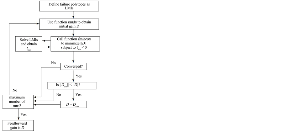
Figure 1. Flowchart for design of feedforward gain using MATLABLMI and Optimization toolboxes.
moving on to another initial condition and a new optimization run. This process is repeated until the maximum number of runs has been reached, at the end of which, D is the gain that makes the plant and the failed plants MP. For the examples in the next section we perform 300 optimization runs with 9999 iterations each.
It is important to note that by considering an LMI set consisting of a single polytope corresponding to a failure in one control effector, and using the D obtained from the optimization, we can increase the percentage of loss of control effectiveness in steps of 0.1 and check if the feasibility of the LMI set is maintained for additional percentage failure. Depending on the type of failure, the D may or may not allow more loss of control effectiveness than the amount that was initially defined for each failure.
We remark that when searching for a D for plants with a single failure in any one control effector, the LMI set in design process can be defined to include only one polytope at a time. This would require, however, finding a different D for each type of effector failure and so we would be forced to first identify the failure in order to use the appropriate feedforward gain. Furthermore, no claims are made about the convergence rate and optimality of the proposed feedforward design process.
9. Examples
9.1. F/A-18 Aircraft
9.1.1. F/A-18 Aircraft and Reference Model
Consider the linearized lateral dynamics of the F/A-18 aircraft described in [12] . The rigid body states are lateral velocity v (ft/s), yaw rate r (deg/s), roll rate p (deg/s), and bank angle  (deg). The control surface deflections are asymmetric trailing edge flaps
  (deg), ailerons
  (deg), and rudder
  (deg). The deflection limits, taken to be the same as those for the F-16 aircraft [29] , are
 ,
,  , and
, and . The deflection rate limits are
  (deg/s),
  (deg/s), and
  (deg/s). The measurements are sideslip angle
  (deg), washed out yaw rate
  (deg), and roll rate p (deg/s). The unfailed aircraft is described by the triple
 , where the matrices
  and
and  are shown in [12] .
The continuous time model  is converted to the delta model using the c2del function from the MATLAB Delta Toolbox with a sampling rate of 200 Hz. Here we use the same output feedback delta domain gain matrix
  from [16] shown in Table 1, which was designed using eigenstructure assignment for the unfailed aircraft. This constant output feedback gain will be placed around both the aircraft and the reference model. Thus, the adaptive algorithm will control the closed loop aircraft. The block diagram of the adaptive control system is shown in Figure 2.
Barkana, Rusnak, and Weiss [19] have shown that a constant parallel feedforward gain D can be implemented as part of the adaptive controller. Therefore, nothing is added in parallel with the aircraft in the implementation of the adaptive controller. However, the gain D does create an algebraic loop. Barkana, Rusnak, and Weiss [19] eliminate the algebraic loop by using the augmented error  to compute the adaptive gain
  in Equation (18) and then using its value to obtain the adaptive control signal in the form
 (41)
(41)
As shown in Figure 3. The equivalence between Figure 2 and Figure 3 is shown in detail in [19] . Therefore,

Table 1. Eigenstructure assignment gain for the F/A-18 aircraft from Belkharraz and Sobel [16] .
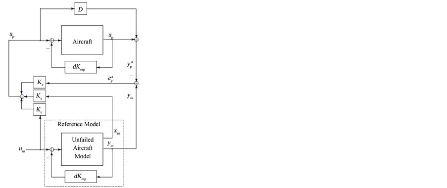
Figure 2. Block diagram of the simple adaptive controller for accomodation of aircraft loss of control effectiveness failures.

Figure 3. Block diagram of the implementation of the simple adaptive controller without algebraic loop.
the computer simulations of the adaptive controllers for the two aircraft examples presented in this paper do not add anything in parallel with the aircraft.
The closed loop unfailed aircraft (plant) in the delta domain is described by the triple
 . We choose the reference model to be the same triple. Namely,
 ,
,  , and
, and  so that, when there are no failures, the reference model is exactly the unfailed aircraft with eigenstructure feedback
 . The reference model input
  is given as
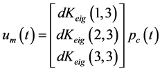 (42)
(42)
where  is the pilot roll rate command described by
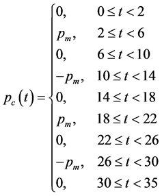 (43)
(43)
and  is the magnitude of the roll rate pulse in deg/sec.
9.1.2. Bounded Input Disturbance
In this example we consider a bounded input disturbance in the form of a lateral gust , which is described in [16] and given by
 (44)
(44)
where  are the instants at which the disturbance occurs and where
  is the lateral gust magnitude. The gust length T is chosen to be to be the inverse of the natural frequency
  of the closed loop complex eigenvalue pair of the unfailed aircraft. Here the dutch roll eigenvalues are
  so that
 sec.
sec.
9.1.3. Feedforward Gain for the F/A-18 Aircraft
For the F/A-18 aircraft there are a set of five LMIs. These include 1) an LMI representing the unfailed aircraft, 2) an LMI for positive definite P, and 3) three LMIs for the three failure polytopes. Each of the three failure polytopes has two vertices with one vertex for the unfailed aircraft and a second vertex for the aircraft with one control effector failure. So the three failure LMIs represent a) the aircraft with a failure in the trailing edge flaps, b) the aircraft with a failure in the ailerons, and c) the aircraft with a rudder failure. Belkharraz and Sobel [16] used an 80% effectiveness failure in any one control effector, and so we choose each of the failed vertices for the F/A-18 aircraft to be defined with an 80% loss of control effectiveness. Using our proposed method with a sampling rate of 200 Hz, we found the feedforward gain matrix D shown in Table 2 that has a Frobenius norm of 0.0889. This feedforward gain was obtained by choosing the D with minimum Frobenius norm from among those D matrices with positive definite P. Out of the 300 optimization runs, 16 converged to a feasible feedforward gain; the maximum Frobenius norm was 0.8457.
Table 2. Feedforward gain for the F/A-18 aircraft.
Once the gain D was found, we considered each of the three two-vertex polytopes that include the unfailed aircraft and the aircraft with one control effector failure. By modifying our LMI program to include only three LMI’s (one for the unfailed aircraft, one for the aircraft with one failure, and one for the  constraint) we search for a positive definite P with the same feedforward matrix obtained in the previous optimization. Clearly, when the effectiveness failure is at most 80%, a feasible solution to the new system of LMI's is guaranteed to exist. However, if we keep increasing the effectiveness failure in steps of 0.1 we find that the single failed F/A-18 aircraft remains minimum-phase for a 92% trailing edge flap failure, a 99% aileron failure, and a 80% rudder failure.
9.1.4. Weighting Matrices for the F/A-18 Aircraft
We now describe our selection process for the weighting matrices for the F/A-18 aircraft using a computer simulation with the reference model input in Equation (42), but without the lateral gust in Equation (44). In order to simplify the approach, we first let  and T be diagonal matrices and also let
 . We then take our first set of candidates to be
 . A computer simulation for this candidate shows no acceptable tracking of the reference model for the first 20 seconds of the simulation and so it is rejected. We then choose to make the weights for the
 ’s (the first three entries in
  and T) larger. That is, we choose our second set of candidates as
 . A computer simulation for this candidate shows acceptable tracking everywhere except at
  sec where there is an unacceptable jump which results from an unrealistic deflection rate in the control signals, and so it is rejected. We now let
  and recall that
  is the weighting matrix for the proportional part of the adaptive algorithm. Therefore, we make an effort to have the entries of
  be smaller than those of T. This is because we want to avoid having any jumps from appearing in the simulation. To this end we choose our third set of candidates to be
  and
and . A computer simulation shows that although its magnitude has been decreased, the jump in the response still persists, and so we reject it. Thus we again choose to change the entries of
 and so our fourth set of candidates is taken to be
  and
and . The computer simulation shows that the jump has almost disappeared but not completely. We note that the jump is larger in the roll rate output and so we choose to modify the third entry of T, which is the weighting entry for the roll rate measurement. Thus we take
 and
and  as our fifth set of candidates. The computer simulation shows the best tracking performance of all attempts. However, we see some undesirable high frequency oscillations in the measurements. Now that we have a good set of candidates for the weighting matrices, we attempt to eliminate the oscillation by modifying the other entries of the matrices. To this end we let
 and
and be our sixth set of candidates. A computer simulation shows that the oscillation is reduced considerably and so we proceed again to further decrease the weights for the
 ’s in each matrix until the oscillation completely disappears. Thus we arrive at our final choice for
  and T as
 and
and
 .
.
9.1.5. Simulation Results for the F/A-18 Aircraft
We perform non-adaptive simulations with the fixed gain controller  for the F/A-18 aircraft with
 . The single control effector failures occur at
  sec. A wind gust of magnitude
  (ft/s), as described in Equation (44), occurs at
  sec and has a duration of 10sec. The non-adaptive simulation corresponds to letting
 , and also omitting D. Both reference model and aircraft have zero initial conditions. The non-adaptive time responses are shown on the left side of Figure 4, where the black line corresponds to the reference model, the red line corresponds to a 92% trailing edge flap failure, the green line corresponds to a 99% aileron failure, and the blue line corresponds to a 80% rudder failure. Observe the unacceptable tracking performance in sideslip angle
 , yaw rate r, and roll rate p for each surface failure. Furthermore, the coordinated turn is not achieved when an aileron failure occurs. Recall that here we feed back the washed out yaw rate
  (deg/s), but we plot the true yaw rate r (deg/s).
Finally, we perform adaptive simulations of the F/A-18 to accommodate the same surface failures and input disturbance using the proposed adaptive controller with feedforward matrix D as given in Table 2. The weighting matrices used in the simulation are the same as those obtained above for the unfailed adaptive response. Here we let . The adaptive time responses are shown on the right side of Figure 4. The adaptive control surface deflections are rate limited. Observe the almost perfect tracking in sideslip angle
 , yaw rate r, and roll rate p.
9.2. Tailless Aircraft
9.2.1. Tailless Aircraft and Reference Model
We now consider the linearized dynamics of the Innovative Control Effectors (ICE) aircraft which was described in Nieto-Wire and Sobel [20] . The state variables are velocity  (ft/s), angle of attack
  (rad), pitch angle
  (rad), pitch rate q (rad/s), engine power level, sideslip angle
  (rad), bank angle
  (rad), roll rate p (rad/s), and yaw rate r (rad/s). The control effectors are throttle
  (0-1), symmetric pitch flap
  (deg), left elevon
  (deg), right elevon
  (deg), left all moving tip
  (deg), right all moving tip
  (deg), pitch thrust vectoring
  (deg), and yaw thrust vectoring
  (deg). The deflection limits are
 ,
, ,
,  ,
,  ,
, . The deflection rate limits are
  deg/s,
  deg/s,
  deg/s,
  deg/s,
  deg/s.
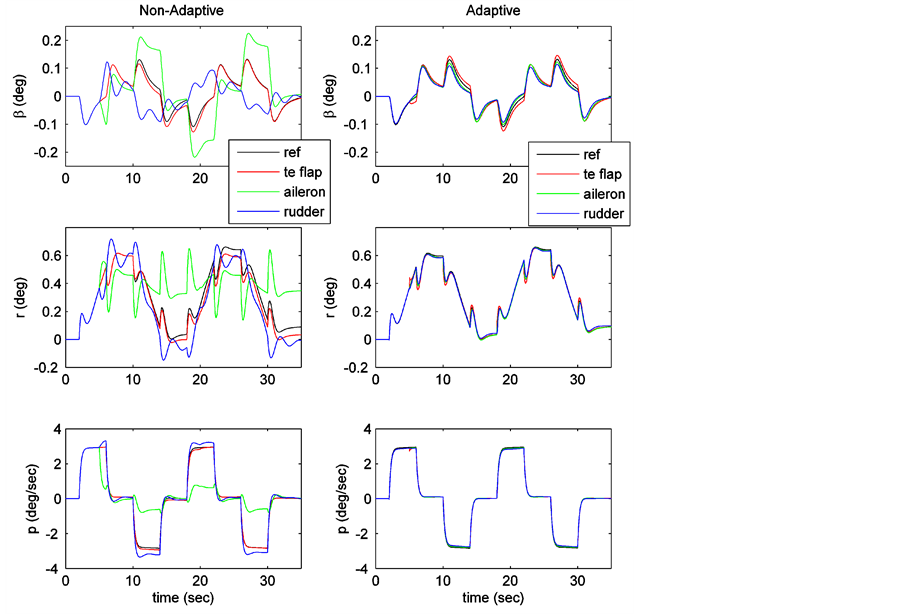
Figure 4. FA/18 Aircraft at 200 Hz. Failures at t = 5 sec: 92% trailing edge flap, 99% aileron, and 80% rudder failures. 15 fps lateral wind gust disturbance at t = 10 sec with duration of 10 sec.
In this example we consider the linearized lateral dynamics. The lateral control effectors are left elevon  (deg), right elevon
  (deg), left all moving tip
  (deg), right all moving tip
  (deg), and yaw thrust vectoring
  (deg). The sensor measurements are sideslip angle
  (deg), roll rate p (deg/s), and yaw rate r (deg/s). Nieto-Wire and Sobel [20] transformed the lateral dynamics from body axis to stability axis so that stability axis roll rate
  could be decoupled from sideslip angle. For the transformation the value of trim alpha used is 0.1569 rad. The states are now sideslip angle
 , bank angle
 , stability axis roll rate
 , stability axis yaw rate
 , and a washout filter state
 . The lateral feedbacks are chosen to be
 ,
,  , and washed
out stability axis yaw rate .
.
The unfailed continuous time aircraft model is described by the triple  where the matrices
 ,
,  , and
, and  are given in [20] . The continuous time model for the ICE aircraft is converted to the delta model by using the c2del function from the MATLAB Delta Toolbox with a sampling rate of 1 kHz. We use the method proposed in [20] to compute the eigenstructure assignment gain
  for the unfailed aircraft which is shown in Table 3. We assign the desired dutch roll damping ratio
 , natural frequency
 , and roll subsidence eigenvalues as
 ,
,  , and
, and . This constant output feedback gain
  will be placed around both the aircraft and the reference model. Thus, the adaptive algorithm will control the closed loop aircraft.
The closed loop unfailed aircraft in the delta domain with eigenstructure assignment is described by the triple
 . The reference model is chosen to be the same triple so that
 ,
,  ,
, . Thus, when there are no failures the reference model is the aircraft with eigenstructure assignment gain
 . The reference model input
  is given as
 (45)
(45)
where  is the pilot roll rate command given in Equation (43). The 4/3 gain in
  has been added to the pilot stick for the purpose of achieving zero steady-state error to a
  command.
9.2.2. Feedforward Gain for the Tailless Aircraft
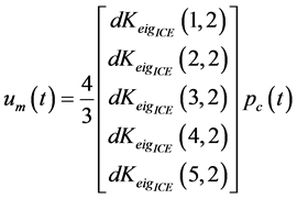
In this example we consider loss of control effectiveness failures in any one control effector. Here we add bank angle feedback in the implementation of the adaptive controller only. We linearly map the five lateral control effectors into four, and use left and right elevons, the all moving tips, and yaw thrust vectoring to yield a total of four control surfaces. That is, we map left and right all moving tips into a single control signal as:
 . This is done because our adaptive algorithm requires that the number of inputs equal the number of outputs. We also require that the failures be symmetric; otherwise cross coupling effects between the lateral and longitudinal axes must be considered.
Table 3. Eigenstructure assignment gain for the tailless aircraft using a sampling rate of 1 kHz.
For the tailless aircraft we define a set of five LMIs. These include 1) an LMI representing the unfailed aircraft, 2) an LMI for positive definite P, and 3) three LMIs for the three failure polytopes. Each of the three failure polytopes has two vertices with one vertex for the unfailed aircraft and a second vertex for the aircraft with one control effector failure. So the three failure LMIs represent a) the aircraft with a failure in the elevons, b) the aircraft with a failure in the all moving tips, and c) the aircraft with a yaw thrust vectoring failure. Since we do not know in advance how much loss of control effectiveness can be effectively accommodated by the adaptive controller, we choose each of the failed vertices for the tailless aircraft to be defined with a 50% loss of control effectiveness. Using our proposed method with a sampling rate of 1 kHz, we found the feedforward gain matrix D shown in Table 4 that has a Frobenius norm of 0.0043. This feedforward gain was obtained by choosing the D with minimum Frobenius norm from among those D matrices with positive definite P using 300 optimization runs. Out of the 300 optimization runs, 29 converged to a feasible feedforward gain; the maximum Frobenius norm was 4.3351.
In this case increasing the percentage of loss of control effectiveness failure for each polytope individually, with the D obtained from the optimization, does not yield feasible LMIs beyond 50%.
9.2.3. Weighting Matrices for the Tailless Aircraft
An approach similar to that described for obtaining the weights for the adaptive algorithm in the FA-18 aircraft example yields the weights .
.
9.2.4. Simulation Results for the Tailless Aircraft
We now perform computer simulations using the ICE model for different control effector failures. Consider the roll rate pilot command  is given by Equation (43). We first perform non-adaptive simulations with the fixed gain controller
  for the ICE aircraft with
 . The single control effector failures occur at
 sec. In this simulation we do not include a wind gust disturbance. The non-adaptive simulation corresponds to letting
 , and also omitting D. Both reference model and aircraft have zero initial conditions. The non-adaptive time responses are shown on the left side of Figure 5, where the black line corresponds to the reference model time response, the red line corresponds to a 50% elevon failure, the green line corresponds to a 50% all moving tip failure, and the blue line corresponds to a 50% yaw thrust vectoring failure. Observe the poor tracking performance in sideslip angle
 , stability axis yaw rate
 , and stability axis roll rate
  for each surface failure. Recall that we feed back the washed out stability axis yaw rate
  (deg/s) but here we plot the stability axis yaw rate
  (deg/s).
Next we perform adaptive simulations of the ICE aircraft to accommodate the surface failures and input disturbance using the proposed adaptive controller with feedforward matrix D as given in Table 4. We initialize the adaptive gains as , which corresponds to initializing the failed plant with the eigenstructure assignment feedback which was designed for the unfailed aircraft. Here we combine the five lateral control signals from
  into four signals that go into the adaptive controls. The adaptive algorithm yields four adaptive control signals which are then mapped back into five control signals for the tailless aircraft. The amount of failure and weighting matrices used in the adaptive simulation are the same as those used in the non-adaptive simulation. Here we let
 . The adaptive time histories are shown on the right side of Figure 5. The adaptive control surface deflections are rate limited. Observe the almost perfect tracking performance of the adaptive controller in sideslip angle
 , stability axis yaw rate
 , and stability axis roll rate
Table 4. Feedforward gain for the tailless aircraft using a sampling rate of 1 kHz.

Figure 5. Tailless Aircraft at 1 kHz. Failures at t = 5 sec: 50% in any one control effector. No wind gust disturbance.
for each control effector failure.
For the following set of simulations we introduce a wind gust disturbance of magnitude  (ft/s) as described in Equation (44), which occurs at
  sec and has a duration of 10 sec. The gust length T in Equation (44) is chosen to be to be the inverse of the natural frequency
  of the closed loop complex eigenvalue pair of the unfailed aircraft; here
  so that
  sec. Here the amount of failure and weighting matrices are the same as those used in the simulations of Figure 5. The non-adaptive time responses are shown on the left side of Figure 6, where the black line corresponds to the reference model time response, the red line corresponds to a 50% elevon failure, the green line corresponds to a 50% all moving tip failure, and the blue line corresponds to a 50% yaw thrust vectoring failure. By comparing the left sides of Figure 5 and Figure 6, we can clearly see that the fixed controller performance deteriorates considerably due to the disturbance. Observe how the fixed controller, on the left side of Figure 6, starts diverging once the wind gust occurs, as can be seen in the bank angle and yaw rate outputs, and does not recover. Compare this to the response of the adaptive controller shown in the right side of Figure 6 which exhibits almost perfect tracking and is able to successfully accommodate considerable loss of control effectiveness failures even in the presence of a bounded lateral wind gust disturbance.
10. Conclusion
A new proof that yields a sufficient condition for stability in the delta domain for simple adaptive control in terms of a linear matrix inequality has been presented. We have shown how to compute a feedforward gain D

Figure 6. Tailless Aircraft at 1 kHz. Failures at t = 5 sec: 50% in any one control effector. 5 fps lateral wind gust disturbance at t = 10 sec with duration of 10 sec.
that makes the augmented plant minimum-phase, and thus ASPR, by defining an LMI set that represents a convex control effector failure polytope. The approach consists of minimizing the Frobenius norm of D subject to LMI constraints. The designs used a fixed eigenstructure assignment controller for an inner loop augmented with the simple adaptive controller. The adaptive algorithm and the proposed method to compute the feedforward gain have been applied to both an F/A-18 aircraft and a tailless aircraft with lateral wind gust disturbances. A feedforward gain was designed for an F/A-18 aircraft for a loss of control effectiveness in any one control effector of 92% trailing edge flap, 99% aileron, or 80% rudder. Furthermore, a feedforward gain was designed for a tailless aircraft for a loss of control effectiveness in any one control effector of 50% elevon, 50% all moving tips, or 50% yaw thrust vectoring. Computer simulations for both aircraft with a failure in any one control effector under lateral gust conditions exhibited almost perfect tracking with the adaptive algorithm whereas the nonadaptive F/A-18 controller could not achieve a coordinated turn when an aileron failure occurred and the nonadaptive tailless aircraft controller diverged when an all moving tip failure occurred.
Cite this paper
Alfredo Cano,Kenneth Sobel, (2016) Simple Adaptive Delta Operator Aircraft Flight Control for Accommodation of Loss of Control Effectiveness. Engineering,08,173-195. doi: 10.4236/eng.2016.84016
References
- 1. Fradkov, A.L. (1976) Quadratic Lyapunov Function in the Adaptive Stabilization Problem of a Linear Dynamic Plant. Siberian Mathematical Journal, 17, 341-348.
http://dx.doi.org/10.1007/BF00967581 - 2. Sobel, K., Kaufman, H. and Mabius, L. (1979) Model Reference Output Adaptive Control Systems without Parameter Identification. 18th IEEE Conference on Decision and Control Including the Symposium on Adaptive Processes, Fort Lauderdale, 12-14 December 1979, 347-351.
http://dx.doi.org/10.1109/cdc.1979.270194 - 3. Sobel, K., Kaufman, H. and Mabius, L. (1982) Adaptive Control for a Class of Mimo Systems. IEEE Transactions on Aerospace and Electronic Systems, 18, 576-590.
http://dx.doi.org/10.1109/TAES.1982.309270 - 4. Barkana, I. (1985) Global Stability and Performance of an Adaptive Control Algorithn. International Journal of Control, 46, 1491-1505.
http://dx.doi.org/10.1080/00207178508933440 - 5. Barkana, I. (1987) Parallel Feedforward and Simplified Adaptive Control. International Journal of Adaptive Control and Signal Processing, 1, 95-102.
http://dx.doi.org/10.1002/acs.4480010202 - 6. Kaufman, H., Barkana, I. and Sobel, K.M. (1998) Direct Adaptive Control Algorithms Theory and Applications. 2nd Edition, Springer-Verlag, New York.
http://dx.doi.org/10.1007/978-1-4612-0657-6 - 7. Mizumoto, I., Fukui, S., Yamanaka, K. and Shah, S.L. (2011) Performance-Driven Adaptive Output Feedback Control System with a PFC Designed via Frit Approach. Proceedings of the 2011 International Conference on Advanced Mechatronic Systems, Zhengzhou, 11-13 August 2011, 331-336.
- 8. Mooij, E. (2014) Passivity Analysis for Nonlinear Nonstationary Entry Capsules. International Journal of Control of Adaptive Control and Signal Processing, 28, 708-731.
http://dx.doi.org/10.1002/acs.2386 - 9. Rusnak, I., Weiss, H. and Barkana, I. (2014) Improving the Performance of Existing Missile Autopilot Using Simple Adaptive Control. International Journal of Control of Adaptive Control and Signal Processing, 28, 732-749.
http://dx.doi.org/10.1002/acs.2457 - 10. Luzi, A.R., Peaucelle, D., Biannic, J.-M., Pittet, C. and Mignot, J. (2014) Decentralized Simple Adaptive Control of Nonlinear Systems. International Journal of Control of Adaptive Control and Signal Processing, 28, 664-685.
http://dx.doi.org/10.1002/acs.2406 - 11. Ulrich, S. and Sasiadek, J. (2014) Decentralized Simple Adaptive Control of Nonlinear Systems. International Journal of Control of Adaptive Control and Signal Processing, 28, 750-763.
http://dx.doi.org/10.1002/acs.2446 - 12. Belkharraz, A.I. and Sobel, K.M. (2003) Direct Adaptive Control for Aircraft Control Surface Failures. Proceedings of the American Control Conference, Denver, 4-6 June 2003, 3905-3910.
http://dx.doi.org/10.1109/acc.2003.1240445 - 13. Belkharraz, A.I. and Sobel, K.M. (2007) Simple Adaptive Control for Aircraft Control Surface Failures. IEEE Transactions on Aerospace and Electronic Systems, 43, 600-611.
http://dx.doi.org/10.1109/acc.2003.1240445 - 14. Barkana, I. (1989) Absolute Stability and Robust Discrete Adaptive Control of Multivariable Systems. In: Leondes, C.T., Ed., Control and Dynamic Systems—Advances in Theory and Applications, Vol. 31, Academic Press, 157-183.
- 15. Ben Yamin, R., Yaesh, I. and Shaked, U. (2010) Robust Discrete-Time Simple Adaptive Regulation. Systems and Control Letters, 59, 787-791.
http://dx.doi.org/10.1016/j.sysconle.2010.09.005 - 16. Belkharraz, A.I. and Sobel, K.M. (2005) Simple Adaptive Control in the Delta Domain for Aircraft Control Surface Failures. AIAA Paper 2005-6249.
- 17. Middleton, R.H. and Goodwin, G.C. (1990) Digital Control and Estimation: A Unified Approach. Prentice-Hall, Upper Saddle River.
- 18. Balas, G., Chiang, R., Packard, A. and Safonov, M. (2016) Robust Control Toolbox for Use with MATLABR. The Mathworks, Inc, Natick.
http://www.mathworks.com/help/pdf_doc/robust/robust_ug.pdf - 19. Barkana, I., Rusnak, I. and Weiss, H. (2014) Almost Passivity and Simple Adaptive Control in Discrete-Time Systems. Asian Journal of Control, 16, 947-958.
http://dx.doi.org/10.1002/asjc.771 - 20. Nieto-Wire, C. and Sobel, K.M. (2009) Reconfigurable Delta Operator Eigenstructure Assignment for a Tailless Aircraft. AIAA Paper 2009-6306.
- 21. Cano Martinez, A. and Sobel, K. (2014) Simple Adaptive Control in the Delta Domain Using a Linear Matrix Inequality. Proceedings of the 2014 AIAA Guidance, Navigation, and Control Conference, National Harbor, 13-17 January 2014.
http://dx.doi.org/10.2514/6.2014-0085 - 22. Ioannou, P. and Kokotovic, P. (1983) Adaptive Systems with Reduced Models. Springer-Verlag, Berlin.
http://dx.doi.org/10.1007/BFb0006357 - 23. Collins, E.G., Haddad, W.M., Chellaboina, V. and Song, T. (1997) Robustness Analysis in the Delta Domain Using Fized-Structure Multipliers. IEEE Conference on Decision and Control, 4, 3286-3291.
- 24. Kottenstette, N. and Antsaklis, P.J. (2010) Relationships between Positive Real, Passive Dissipative, and Positive Systems. Proceedings of the 2010 American Control Conference, Baltimore, 30 June-2 July 2010, 409-416.
http://dx.doi.org/10.1109/acc.2010.5530779 - 25. Duan, G.R. and Yu. H.H. (2013) LMIs in Control Systems: Analysis, Design and Applications. CRC Press, Boca Raton.
- 26. Kouvaritakis, B. and MacFarlane, A.G.J. (1976) Geometric Approach to Analysis and Synthesis of System Zeros. Part 1. Square Systems. International Journal of Control, 23, 149-166.
http://dx.doi.org/10.1080/00207177608922149 - 27. Branch, M.A. and Grace, A. (1996) Optimization Toolbox User’s Guide MATLABR. The Mathworks, Inc, Natick.
- 28. Pascal, G., Arkadi, N., Alan, L. and Mahmoud, C. (1995) LMI Control Toolbox for Use with MATLABR. The Mathworks, Inc, Natick.
- 29. Brian, L.S. and Frank, L.L. (1992) Aircraft Control and Simulation. John Wiley & Sons, Inc., Hoboken.
Appendix
A.1. Preliminary Result: Closed Loop System Equations
The closed loop system is given by [21]
 (46)
(46)
 (47)
(47)
where ,
,  ,
,  ,
,  , and
, and
 .
.
A.2. Proof of Theorem 1
Select a positive quadratic Lyapunov function  such that its derivative
  is negative definite for some
  for
for . The Lyapunov candidate must include all dynamic values
  and
and  of the system, namely
 (48)
(48)
Note that ,
,  for all
 , and
, and  as
as or
or .Applying the unified operator to Equation (48) along the trajectories of system in Equations (46)-(47) results in

 can be written as follows [21] :

Then,
 (49)
(49)
where
 (50)
(50)
where
 (51)
(51)
and

 can be written as follows [21] :
 (52)
(52)
If the system in Equations (46)-(47) is ASPR, then  which implies
 . Using an analysis similar to appendix 4A in Kaufman, Barkana, and Sobel [6] , we first consider the trajectories where
  remains bounded while
  and
and  increase without bound. Recall that the components
 ,
,  , and
, and  are bounded because the reference model and the input disturbance are assumed to be bounded, then there exist positive constants
 , and
, and  such that
 (53)
(53)
For any real numbers x and y there exists some positive finite scalars , and
, and  such that
 (54)
(54)
 (55)
(55)
 (56)
(56)
 (57)
(57)
Then using Equations (54)-(57) we have
 (58)
(58)
or

Let  then
then
 (59)
(59)
We can see from Equation (59) that if , then
  is negative.
Observe that there exist some positive finite constants , and
, and  such that
 (60)
(60)
which implies that . Since
  is positive, this implies
  for any
 and for some
 . Hence
  for any
  and for some
 .
.
Now consider the trajectories where  together with
  and
and  increase without bound. We have that
 (61)
(61)
There exist positive constants , and
, and  such that
 (62)
(62)
Rewrite Equation (62) as
 (63)
(63)
or
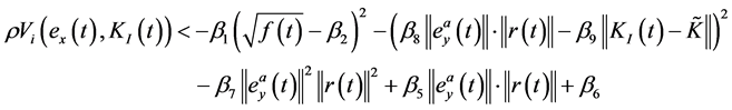 (64)
(64)
For some value  such that
  the first two negative terms in Equation (64) together with
 will dominate the positive terms of lesser degree. This implies that
 for any
  and for any
 .
.
Therefore,  for any
  and
and  which guarantees that all adaptation variables are bounded.
NOTES

*Corresponding author.