Engineering
Vol.5 No.10A(2013), Article ID:37226,8 pages DOI:10.4236/eng.2013.510A001
Load Flow Analysis Framework for Active Distribution Networks Based on Smart Meter Reading System
Department of Electrical Engineering, Aalto University, Espoo, Finland
Email: merkebu.degefa@aalto.fi;john.millar@aalto.fi; matti.koivisto@aalto.fi; muhammad.humayun@aalto.fi; matti.lehtonen@aalto.fi
Copyright © 2013 Merkebu Zenebe Degefa et al. This is an open access article distributed under the Creative Commons Attribution License, which permits unrestricted use, distribution, and reproduction in any medium, provided the original work is properly cited.
Received June 16, 2013; revised July 13, 2013; accepted July 20, 2013
Keywords: Active Network; Demand Response; Dynamic Rating; Load Forecast; Load Modeling; Smart Meter; State Estimation
ABSTRACT
With the expansion of distributed generation systems and demand response programs, the need to fully utilize distribution system capacity has increased. In addition, the potential bidirectional flow of power on distribution networks demands voltage visibility and control at all voltage levels. Distribution system state estimations, however, have traditionally been less prioritized due to the lack of enough measurement points while being the major role player in knowing the real-time system states of active distribution networks. The advent of smart meters at LV loads, on the other hand, is giving relief to this shortcoming. This study explores the potential of bottom up load flow analysis based on customer level Automatic Meter Reading (AMRs) to compute short time forecasts of demands and distribution network system states. A state estimation frame-work, which makes use of available AMR data, is proposed and discussed.
1. Introduction
Distribution system state estimation provides the realtime system states to a Distribution Management System (DMS) enabling operators to monitor and control the operation of the distribution system. With the transformation of distribution networks from passive networks to active networks, following widespread installations of Distributed Generation (DG) and Smart Metering (SM) technologies, the state estimation tool is becoming a core component. In fact, this tool has been used widely and for a long time with transmission systems. The utilization of the tool in distribution systems has been lagging due to two reasons: the first was the absence of widespread measurement, in distribution networks and the second is the low need for active management of the distribution network. Nowadays, however, smart meters are being installed down to the customer level opening up the network for more visibility. Nowadays, for effective DG and demand response applications, knowledge and regulation of voltage levels at every node of the active networks is becoming crucial [1-3]. In addition, state estimation has a central benefit in enabling the full utilization of distribution system capacity [4].
A load modeling procedure is a requirement of any distribution circuit state estimator. Load modeling techniques provide real-time estimates of customer load demands.
There has also been the emergence of innovative ideas from power load serving entities to increase efficiency, utilize assets to their utmost, and provide targeted customer services. The consequent impacts on feeder level load profile and diversity, however, are not known yet. The question of how far the peak load can be brought down still needs addressing. Therefore, the empirically driven, non-interactive load models need to give way to sophisticated models that simulate the independent behavior of those components that contribute to the feeder load shape [5].
With the expansion of ICT infrastructure and the advent of smart meters, network information such as connectivity and measurement data are assumed to be readily available in real time. Therefore, a load flow analysis can effectively utilize both the component based and measurement based load modeling outputs as shown in Figure 1.
In this study customer level AMR meter reading is used to build day-after curves of LV node voltages and power. The impact of load modeling at different node points in the network on the load flow analysis is also compared. This paper formulates and proposes a distribution system load modeling framework based on AMR metered consumption data. The potential of detailed customer level load modeling built up from component modeling is discussed.
This paper presents observations from the application of the three building blocks of an active distribution network state estimation framework as shown in Figure 1. Section 2 presents the load modeling techniques and their relevance in today’s active distribution network. Section 3 presents the test network used in this study, which has the topology and configuration of a typical Finnish sub-urban distribution network. The ARX modelbased one day ahead load forecasting is explained in Section 4. Section 5 formulates and applies a simple AMR metering based load flow analysis technique and the last section will conclude the findings.
2. Load Modeling
In practice, domestic smart meters do not transmit data immediately after measurement or on an hourly basis, at least at the time of this study. State estimation is therefore most likely to depend on the previous day’s measurement, requiring the application of very short time load forecasting, especially for the next day. Before performing a load flow analysis or any sort of load estimation and forecasting, one has to model the consumer load. The term “load model” is, however, used both for component based and measurement based load models of the distribution system. Before continuing, we would like to clarify these definitions.
2.1. Component Based Load Modeling
This models customer loads as different component based load types explaining the relationship between the

Figure 1. A state estimation framework for an active distribution network.
power, voltage and current [6,7]. It is usually referred to as a ZIP model, with constant Impedance (Z), Current (I) or Power (P). This modeling technique is explained and formulated in Table 1. In fact, the ZIP model may also be expanded by adding an exponential load type, where the load power varies with the voltage magnitude in an exponential relationship. The general voltage-load current characteristic is plotted in Figure 2.
According to [7], residential areas have a ratio of constant power/constant impedance of 70/30 in strong summer peaking and 30/70 in winter peaking days. In the coming sections the component based modeling used in the load flow analysis is presented. Section 3 presents the component load model of a typical Finnish household.
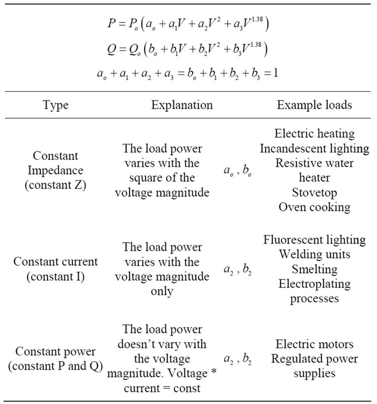
Table 1. Component based load modeling [6].
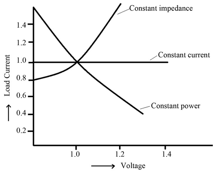
Figure 2. V-I characteristics curves for ZIP model.
2.2. Measurement Based Load Modeling
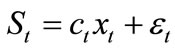
This establishes a relationship between certain independent variables such as weather conditions, the day type and the total load. It aims to extract regression coefficients from static past data for possible future forecasting. These models could also incorporate dynamic behavior such as in ARMAX (Auto Regressive Moving Average and Explanatory variable (X)). The multiple regressions in (1) explain the formulation of such modeling [8].
 (1)
(1)
where
 measured system load datat sampling time,
 vector of adapted variables such as time, temperature, light intensity, wind speed, humidity, day type (workday, weekend), etc.,
 regression coefficients, and
 model error at time t.
Households belonging to the direct electric heating group, for instance, will have different regression coefficients to those belonging to the district heating group. The target of this load modeling type is estimating unmeasured load points based on statistical information and other variable measurements, or forecasting future load. A pure time series model with no additional explanatory variables is proposed in [9], as shown in (2).
 (2)
(2)
The model in (2) requires the past hour consumption of customer i. Smart meters, however, collect electricity consumption data at half hour or one hour intervals and this metering data will be sent to the utility the following day. The model proposed in [9] would not be practical in today’s infrastructure. With one day data delay other time series models such as Autoregressive Moving-Average (ARMA) and Autoregressive Integrated MovingAverage (ARIMA) will also fail to keep up with the dynamism of the load [8]. These models start to lose their relevance as they tend to depend on their own previous hour estimations. We applied the ARX (Auto Regressive with eXogeneous input) model, which utilizes previous day AMR metered consumption data as well as same day explanatory variables such as temperature, day structure, humidity, etc. Section 4 presents the detailed formulation of the ARX model.
2.3. The State Estimation Framework
The state estimation framework presented in Figure1 consists of three fundamental functions: the measurement based modeling, the component based modeling and the load flow analysis. The measurement based modeling explained in Section 2.2 provides real time or near future forecasts of the loading situation while the component based modeling in Section 2.1 is used to undertake an effective and detailed load flow analysis by translating nodal power demand to voltage magnitude and phase (see Figure 1). Not being limited to hourly metered household consumption the framework in Figure 1 proposes a more detailed load flow analysis based on component level consumptions. The load-voltage characteristics will be comprehensive in including the special characteristics of certain load types with voltage; besides, the disaggregated load is essential for real-time and proactive demand response programs [10].
Load disaggregation is also needed for component based modeling. However, since the resolution of AMR metering is usually 15 minutes or above, the use of load disaggregation techniques through feature recognition (Non-Intrusive Load Monitoring systems) are not practical options. Statistical load analysis techniques such as Conditional Demand Analysis (CDA), on the other hand, can be used to disaggregate measurements at connection boxes to individual appliances as long as a detailed appliance survey is undertaken in the area, at least for sample households [11]. Using the CDA technique the household hourly metered kWh can be disaggregated into major appliance consumptions, which can consequently be grouped under the ZIP classification of loads shown in Table 1.
In this study we do not include component based modeling from the disaggregation results of the CDA technique applied to certain Finnish households. Nevertheless, measurement based modeling is applied and explained in section 4.The load flow analysis without the inclusion of component level disaggregation is presented in section 5. We believe, in this study, the introduction of a framework for load flow analysis and the presentation of illustrative applications will at least indicate the possibilities.
3. Test Network
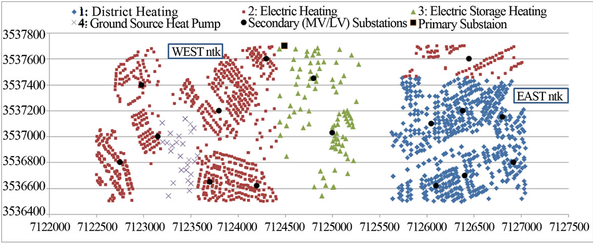
The test network used in this study was laid out by a network planning algorithm capable of producing optimized Greenfield networks or expansion and upgrade plans that utilize existing network. A fully radially operated network without distributed generation is used. However, the motivation of this study, as stated in Section 1, is to utilize load flow analysis techniques and AMR metering data for active distribution network management. The profile of households type connected to the test network is shown in Table 2 and Figure 3 lays out the positions of the household as well as the west side network.
As shown in Table 3, there are 1800 households belonging to one of the four primary heating type groups.
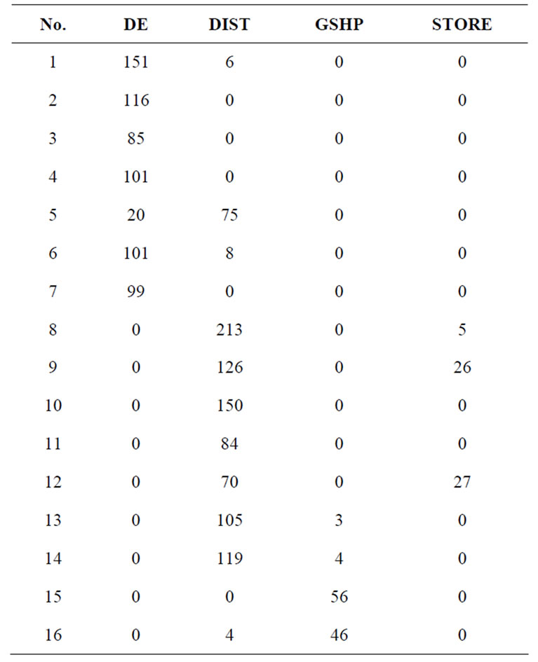
Table 2. Distribution of LV customers of the four heating types under the sixteen secondary substations.
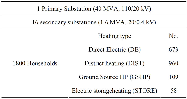
Table 3. Greenfield radial distribution network data.
These households are geographically distributed to build the simulated MV/LV network following geographical boundaries, street grids and the availability of, for example, district heating, as shown in Figure 3(a). On the other hand, we have actual hourly metered consumptions of one year between 2008 and 2009 for the same number of households and heating type profile. For both load forecasting and load flow analysis the actual one year hourly consumptions are randomly assigned to the individual households connected to the simulated network (see Figure 3(b)).
4. One Day Ahead Load Forecasting
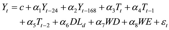
The day ahead load forecasting is based on a simple autoregressive model supported by exogenous variables; it is also called the ARX model. The model has lagging hourly consumption information from the same hour in the previous week and the previous day same hour load, since available measurements are only from the previous day’s metering. The effects of the previous two hours’ temperatures together with real time temperature are included in the explanatory variable. The day structure effect is included through weekday and weekend dummy variables, as shown in (3).
 (3)
(3)
where:
 kWh consumption at hour t
 Temperature at hour t (˚C)
 Day length to represent the light amount of day d
 Weekday dummy variables (0 or 1)
 Weekend dummy variables (0 or 1)
c: Constant
 White noise
The ARX based one day ahead load forecasting is carried out at three points in the network. The parameters 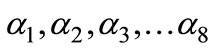 are estimated using an Ordinary Least Squares (OLS) estimator. The results are plotted in Figure 4 and the corresponding Root Mean Square Errors (RMSE) and Mean Absolute Percentage Errors (MAPE) are given for comparison in Table 4.
Case 1:
Forecasting individual customers: Each and every household is modeled individually and a one day ahead forecast is carried out. The consumptions are then aggregated hierarchically at their feeding secondary substation and then the primary substation.
Case 2:
Forecasting at secondary substations: Consumptions of individual households connected to a secondary substation are aggregated before application of the forecasting technique.
Case 3:
Forecasting at the primary substation: All consumptions under the primary substation are aggregated and the aggregated load is modeled and forecasted for the next day.
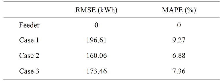
Table 4. RMSE and MAPE comparisons.
 (a)
(a)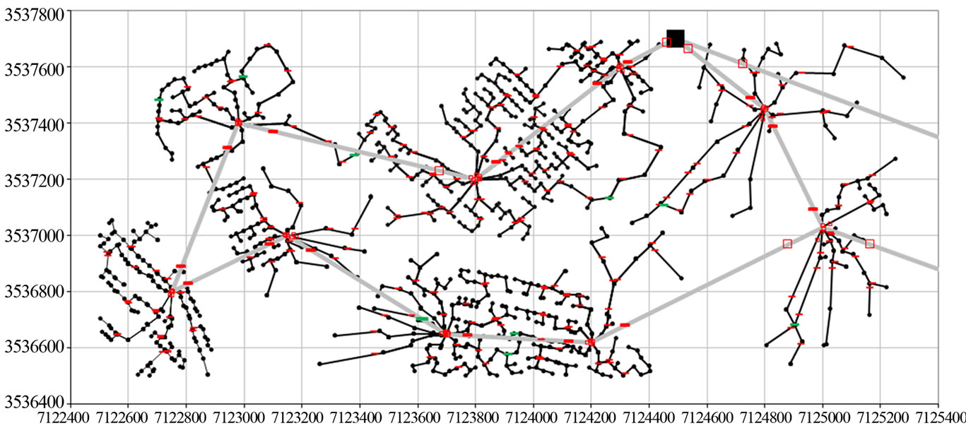 (b)
(b)
Figure 3. The Greenfield test network. (a) Showing the distribution of household types, MV/LV and HV/MV substations; (b) WEST side network.
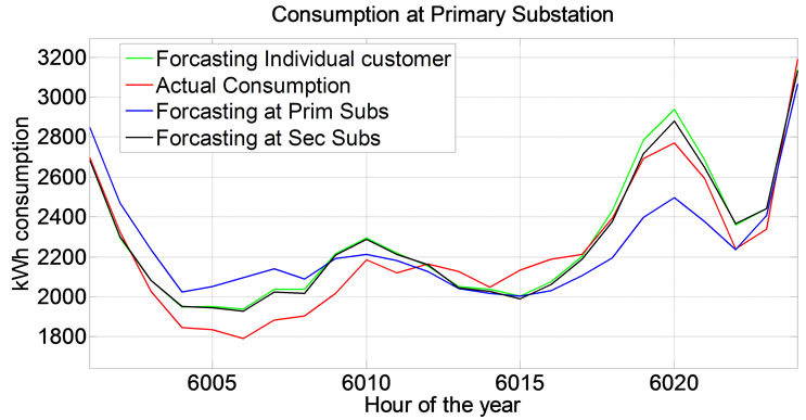
The error is expected to be greater with the attempt to model individual customer level electric loads as these loads do not follow any known distribution function [12]. There is, therefore, a trade-off between the interest in a customer level detailed load flow analysis and obtaining a model with an acceptable error margin. Nevertheless, the results in our study suggest that individual customer level modeling can be attained with a low error difference compared to the secondary substation or primary substation level load modeling (see Table 5 and Figure 4). However, the modeling technique needs to be robust and capable of providing error margins. It has to take into consideration coincidence and correlation factors among individual customers.
5. Load Flow Analysis Based on Customer Level Load Measurement
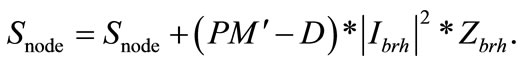
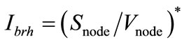
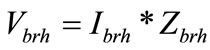
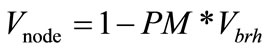
Bidirectional load flow and the integration of DG are the driving forces behind the interest in customer connection point voltage levels in real time. The load flow analysis we implemented uses a simple Backward/Forward sweep technique as formulated in Equations (4) to (7). Due to the different voltage levels a per-unit analysis is used.
 (4)
(4)
 (5)
(5)
 (6)
(6)
 (7)
(7)
where:
 is
is  in kWh at a node
PM: is the node path matrix from the primary substation to every node
D: is a diagonal matrix of equal size to PM
 current flowing on the branch between two nodes (A)
 is the impedance of a branch between two nodes
  (ohms)
 Voltage phasor difference over a branch between two nodes
 voltage level at a node
 Matrix element-by-element multiplication
Including the secondary substations there are 1816 node points in the test network where the voltage magnitude and angle are evaluated.
Results in Figures 5-7 show the hourly voltage profiles of the distribution network up to the LV customer level node. In this load flow analysis no voltage regulation is involved and the results show a cyclic voltage profile following the trend of the power itself. With this
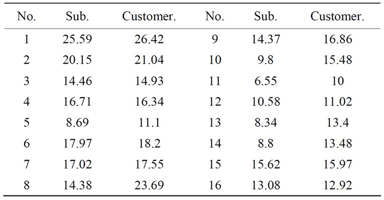
Table 5. RMSE (kWh)comparisons between individual customer forecasts and secondary substation forecasts for the 16 substations.
resolution, the impact of intermittent energy sources such as solar panels can be studied more clearly. As the substation voltage profile in Figure 8 shows, load forecasts of individual customers can be also used to forecast voltage profiles one day ahead. It gets more interesting when forecasts of wind and sun radiation are included together with individual load forecasts to give real-time and one day ahead visibility of the network state.
6. Conclusions and Discussions
Indeed load forecasting at secondary substations experiences lower error than customer level forecasting, as shown in Tables 4 and 5. The quest for customer level voltage visibility, however, requires the redistribution of substation level forecasted load to individual households using statistical information. Referring to the results shown in Tables 4 and 5, it is encouraging that there is little difference in the errors committed when load forecasting is performed at customer points and at secondary substations. The RMSE of voltage forecast using customer forecasted loads was about 0.004 pu and the MAPE is less than 1% (see Figure 8). Therefore customer level load forecasting can be used to conduct load flow analysis giving forecasted customer level voltages.
A load flow analysis based on customer point meter reading can be used to compute LV node voltage levels. The results in Figures 5-7 show meaningful voltages. These results also show that in a traditional suburban distribution network (i.e. without DGs), there seems to be no voltage level problem, as it stayed in the acceptable margin of ±5%.
The component based load modeling which defines the relationship between power and voltage plays a great role in distribution system state estimation. The disaggregation of customer consumption to household appliances is
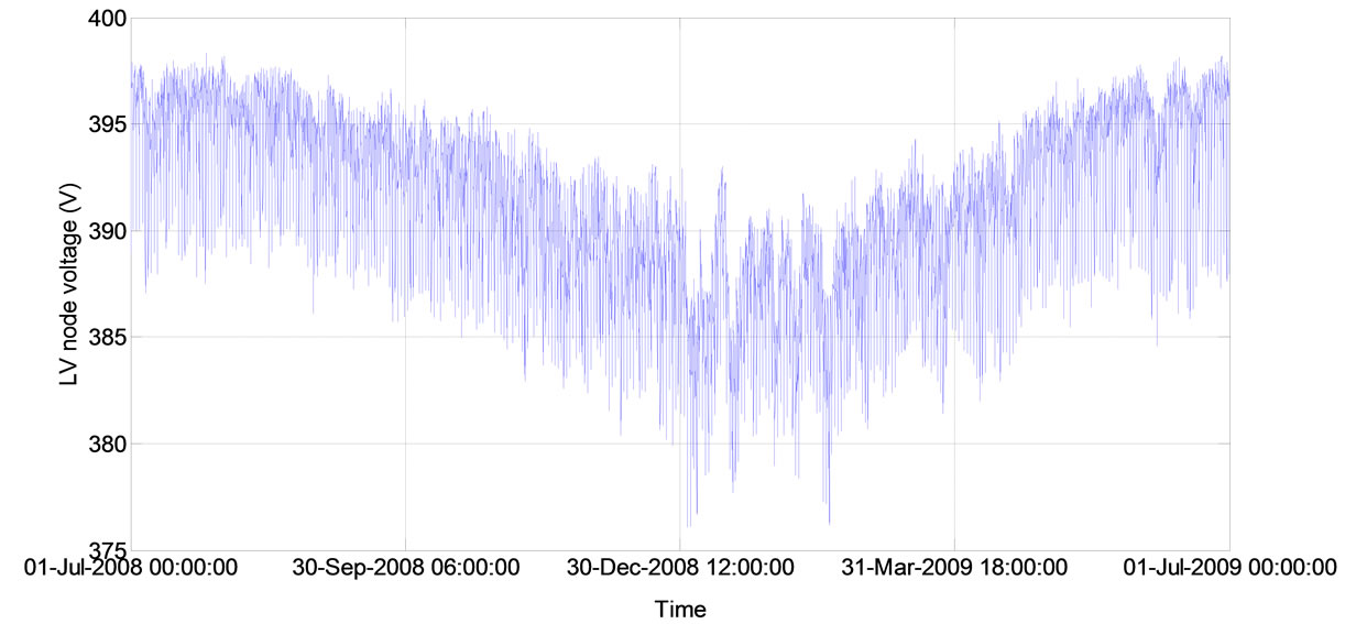
Figure 5. One year hourly voltage profile of the node experiencing the highest voltage drop in the network (MV/LV: 20/0.4 kV). This is without the intrusion of voltage regulation mechanisms such as capacitor banks or tap changing transformers.
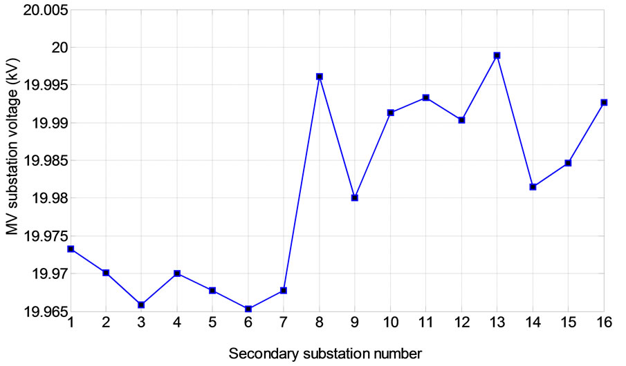
Figure 6. Secondary substation voltages at the hour of the year where the highest voltage drop is experienced at the LV node in Figure 5. (i.e. 01-Jan-2009 23:00:00-00:00:00).
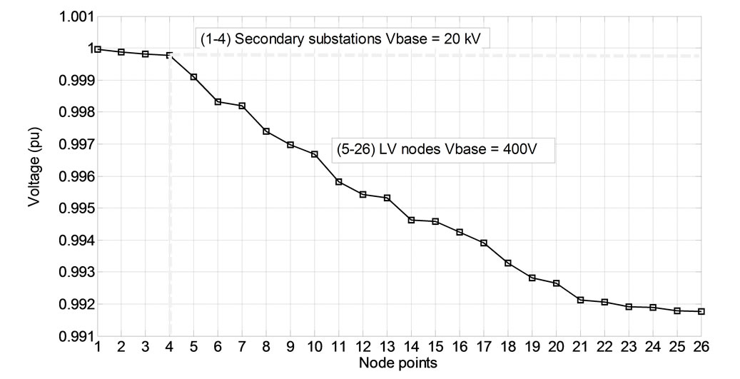
Figure 7. Voltage profile of nodes along the longest path in the network for their mean hourly consumption. On the path there are four secondary substations and 22 LV customers.
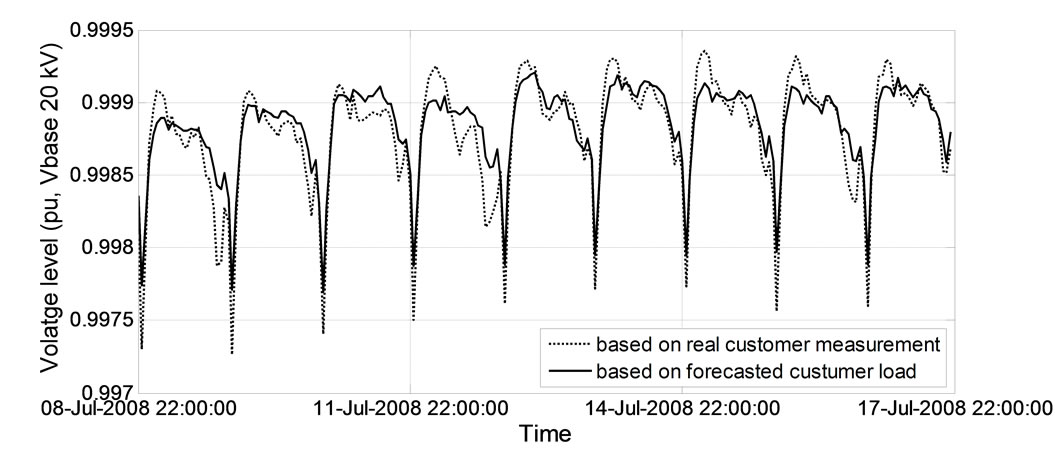
Figure 8. Average voltage profile of the 16 secondary substations for 10 days using real AMR measurement and forecastedcustomer load (Case 1 in Section 4).
the prerequisite for component modeling. Through load disaggregation and component based modeling, the impact of active demand response programs on distribution networks can be viewed more clearly.
In our following research plan, the current network will be expanded to include DGs. Component based modeling will be included in the load flow analysis where the impact of real time demand response programs on the active distribution network will be investigated.
7. Acknowledgements
The authors of this paper would like to acknowledge that this work is supported by the Aalto energy efficiency program through the SAGA project.
REFERENCES
- K. Samarakoon, J. Wu, J. Ekanayake and N. Jenkins, “Use of Delayed Smart Meter Measurements for Distribution State Estimation,” 2011 IEEE Power and Energy Society General Meeting, San Diego, 24-29 July 2011, pp. 1-6.
- A. Abdel-Majeed and M. Braun, “Low Voltage System State Estimation Using Smart Meters,” 47th International Universities Power Engineering Conference (UPEC), London, 4-7 September 2012, pp. 1-6.
- P. A. Pegoraro, J. Tang, J. Liu, F. Ponci, A. Monti and C. Muscas, “PMU and Smart Metering Deployment for State Estimation in Active Distribution Grids,” 2nd IEEE ENERGYCON Conference & Exhibition, Florence, 9-12 September 2012, pp. 873-878.
- M. Lehtonen, M. Jalonen, A. Matsinen, J. Kuru and V. Haapamäki, “A Novel State Estimation Model for Distribution System,” 14th Power Systems Computation Conference PSCC, Sevilla, 24-28 June 2002, pp. 1-5.
- R. T. Guttromson, D. P. Chassin and S. E. Widergren, “Residential Energy Resource Models for Distribution Feeder Simulation,” IEEE Power Engineering Society General Meeting, Toronto, 13-17 July 2003, pp. 108-113.
- K. P. Schneider and J. C. Fuller, “Detailed End Use Load Modeling for Distribution System Analyses,” 2010 IEEE Power and Energy Society General Meeting, Minneapolis, 25-29 July 2010, pp. 1-7.
- H. L. Willis, “Power Distribution Planning Reference Book,” Marcel Dekker, Inc., New York, 1997.
- H. K. Alfares and M. Nazeeruddin, “Electric Load Forecasting: Literature Survey and Classification of Methods,” International Journal of Systems Science, Vol. 33, No. 1, 2002, pp. 23-34.
- H. Wang and N. Schulz, “A Load Modeling Algorithm for Distribution System State Estimation,” IEEE/PES Transmission and Distribution Conference and Exposition Volume 1, Atlanta, 28 October-2 November 2001, pp. 102-105.
- R. F. Arritt, R. C. Dugan, R. W. Uluski and T. F. Weaver, “Investigating Load Estimation Methods with the Use of AMI Metering for Distribution System Analysis,” 2012 IEEE Rural Electric Power Conference (REPC), Milwaukee, 15-17 April 2012, pp. B3-1-B3-9.
- L. G. Swan and V. I. Ugursal, “Modeling of End-Use Energy Consumption in the Residential Sector: A Review of Modeling Techniques,” Elsevier, Renewable and Sustainable Energy Reviews, Vol. 13, No. 8, 2009, pp. 1819- 1835. http://dx.doi.org/10.1016/j.rser.2008.09.033
- A. Seppala, “Statistical Distribution of Customer Load Profiles,” Proceedings of IEEE International Conference on Energy Management and Power Delivery Volume 2, Singapore, 21-23 November 1995, pp. 696-701.