Engineering
Vol. 3 No. 1 (2011) , Article ID: 3715 , 4 pages DOI:10.4236/eng.2011.31001
Reference Coordinate System of Nonlinear Beam Element Based on the Geometrically Exact Formulation under Large Spatial Rotations and Deformations
1Department of Civil Engineering, Auburn University, Auburn, USA
2Department of Civil and Environmental Engineering, Seoul National University, Seoul, Korea (South)
3Zentech Engineering Co. Ltd., Seoul, Korea (South)
4Department of Civil Engineering, Chungbuk National University, Cheongju, Korea (South)
E-mail: kclee@auburn.edu, eclip77@gmail.com
Received September 28, 2010; revised November 29, 2010; accepted December 5, 2010
Keywords: Reference Coordinate System, Element Coordinate System, Large Rotation, Beam Finite Element, Geometric Nonlinearity, Geometrically Exact Beam Formulation
ABSTRACT
Analysis of slender beam structures in a three-dimensional space is widely applicable in mechanical and civil engineering. This paper presents a new procedure to determine the reference coordinate system of a beam element under large rotation and elastic deformation based on a newly introduced physical concept: the zero twist sectional condition, which means that a non-twisted section between two nodes always exists and this section can reasonably be regarded as a reference coordinate system to calculate the internal element forces. This method can avoid the disagreement of the reference coordinates which might occur under large spatial rotations and deformations. Numerical examples given in the paper prove that this procedure guarantees the numerical exactness of the inherent formulation and improves the numerical efficiency, especially under large spatial rotations.
1. Introduction
Long-span bridges, submarine pipelines, flexible aircraft and many other slender structures can be modeled with beam finite elements, which may easily experience large displacements and rotations. These models of slender structures require an advanced geometrical nonlinear analysis to calculate an accurate response for various kinds of design and ultimate load cases. Although fine mesh analysis using solid or shell elements can give good results for these types of structures, beam elements are still gaining popularity in engineering fields because it is simple to model the structures and straightforward to understand the analysis results. Furthermore, it is helpful to adopt them directly into the design process of engineering structures.
Fully nonlinear beam theories have been proposed since 1970, and the representative work was done by Reissner [1] to solve a plane problem. After that, Simo [2] proposed a three-dimensional beam theory, and there are many other implements to analyze geometrically nonlinear beam structures. Beam models of this type have been coined “geometrically exact” because they account for the total deformation and strain without any approximation. Although this approach has been become the dominant approach in the finite element community, the intrinsic difficulty arises from the presence of rotational degrees of freedom and its discretization in the finite element models. This rotational degree of freedom has an intrinsic nonlinear characteristic that makes the formulation and implementation of geometrically exact finite elements complicated. This is more severe in three-dimensional problems, and especially when various rotations are compounded spatially.
In order to keep away from these issues about the rotational degrees of freedom difficulty, the absolute nodal coordinate formulation was recently proposed by Shabana and Yakoub [3,4]. This method employs the element interpolation function, which is generally formed by three interpolation vectors with eight degrees of freedom (DOF). As a result, there are 24 DOFs in one element, this is about twice number of DOFs than a conventional two-noded beam elements implemented by geometrically exact model that has 12 (6 displacements, 6 rotations) or 14 (12 plus each warping per node) DOFs. Although this approach is the only formulation that is not affiliated with rotational variables, it generally costs more computational time than the geometrically exact beam model due to its inherently large number of degrees of freedom. A comparison performed by Romero [5] showed that the geometrically exact model provides more accurate results than the absolute nodal coordinate formulation elements with the same computational cost. In addition, the absolute nodal coordinate formulation cannot sustain the concept of applied moments of loads and imposed rotations; therefore, it is difficult to get a sense of the physical meaning from the analysis results in actual engineering applications. Thus, the most important reason to apply the beam elements might be lessened by using the absolute nodal coordinate formulation.
The geometrically exact beam model is, therefore, still the most accepted approach to analyze slender beam structures involving large rotations and deformations, and the procedure to treat the nonlinear rotational degrees of freedom is valuable to be amended if the numerical performance and exactness of the element can be enhanced. In the geometrically exact beam formulation, a beam is defined as a slender body that can be described mathematically with a centroid curve and a section attached to each point of the curve. The displacement and rotation vectors of each node compose the rotation tensor. The resulting rotation tensor in the reference configuretion defines the deformation of the line of centroids. This configuration is usually called the reference, local or element coordinate system, and the selection of the system is crucial for the general performance of the element when the large rotations and deformations are induced in the nonlinear analysis. This paper first focuses on the prior approaches used to determine the reference coordinate system and identifying a possible lack of physical condition of them under application of large rotations, and later proposes a new procedure to determine the reference coordinate system in order to resolve some of the drawbacks of the existing methods.
For the purpose of comparison, the authors chose two prior methods that were representative of various types of algorithm, proven to work well, and proposed recently. The first was put forward by Crisfield [6,7]; he took a mathematical average to determine the reference coordinate system. The second was suggested by Kuo and Yang [8,9]; they defined the reference coordinate system as the mean vectors of projected axes into the plane perpendicular to the element chord axis. Kuo and Yang adopted an artificial technique in order to establish an orthogonal reference coordinate system based on the property that the diagonals of a rhombus are perpendicular to each other. Other researchers have used similar procedures in order to satisfy the geometrical definition of the Cartesian coordinates. However, all of these procedures do not have logical or mechanical interpretation to determine the reference coordinate system, but rather apply different averaging concepts.
The present paper wants to suggest a new terminology: the zero twist section condition. If rigid body torsional displacements are neglected, a section that is not twisted always exists within an element. This section is named the zero twist section. To guarantee the existence of the zero twist section, the natural torsional deformations of each node in a two-node beam element must always have the same magnitude and opposite sign values. This condition is defined as the Zero Twist Section Condition (ZTSC). When the ZTSC is satisfied, it ensures that the rigid body torsional displacements are uninvolved in a beam formulation and this can be a measure of the faithful implementation of the rotational degrees of freedom.
The large rotations and deformation phenomenon usually works on the post-buckling behavior of frame structures. This study carries out elastic post-buckling analyses of various slender structures that have symmetric, mono-symmetric and non-symmetric cross-sections to induce the spatially combined rotations. For comparison purposes, well-known commercial program ABAQUS beam and solid elements are used to analyze the structures. These comparisons can be a measure of the accuracy and numerical performance of the ZTSC procedure developed in this study.
2. Rotational Tensor and Coordinate System
The Cartesian coordinates system in space is composed of three axes; 1, 2 and 3. A direction cosine ei between an arbitrary i-axis of a coordinate system and the global i-axis gives the vector expressed in (1), which consists of three components ei1, ei2 and ei3. The right subscript denotes the direction of the axis. The left superscript 0 denotes the original un-deformed configuration of the coordinate system, and the superscript 1 stands for the deformed configuration. For the updated Largrangian formulation, this superscript may also be 2. A rotation tensor consists of the direction cosines corresponding to each axis of a coordinate system as given in (2), which becomes a three-by-three matrix in a three-dimensional space.
 (1)
(1)
 (2)
(2)
where, i = 1, 2 and 3, s = 0, 1, or 2.
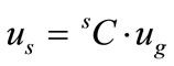
The rotation tensor of a coordinate system sC transforms the reference axes into the local coordinate system from the global one which is expressed as an identity matrix I3. The authors use the same notation sC of the rotation tensor for the coordinate system, because the rotation tensor represents the geometrical configuration of the coordinate system itself. If given values, such as displacements or forces, refer to the global coordinate system, these can be transformed to local values that refer the local coordinate system sC as shown in (3)
 (3)
(3)
where, the subor super-script s (or g) stands for the local (or global) coordinate value, us stands for values whose reference coordinates system is sC.
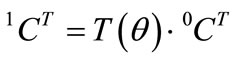
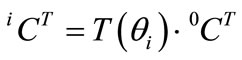
When a spatial rotation θ is imposed in an element at un-deformed configuration 0C, a coordinate system attached to a node is rotated to the deformed configuration 1C. An arbitrary i-axis 0ei of un-deformed coordinate system 0C rotates with a rotation tensor T(θ), which is analytically given by Argyris [10] in Equations (5) and (6). The axis turns into i-axis 1ei of the deformed coordinate system 1C, and then it can be reduced to a single operation as given in (4).
 (4)
(4)
where, 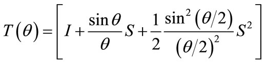 (5)
(5)
 (6)
(6)
This procedure is applied to obtain the deformed nodal coordinate system in a beam element. The deformed nodal coordinate system is represented by 1C and the original un-deformed coordinate system by 0C. Also, the three components of the rotation vector θ are the rotational displacement of a node whose reference axes are the global coordinate system.
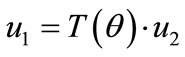
Let us assume the two coordinate systems 1C and 2C, which transform the reference coordinates from the global to local coordinate systems with the 1 and 2 configurations, respectively. These coordinate systems transform the reference of a certain value to their own configurations from the global coordinate system, according to their definitions given in (3). When the reference axes of specific values u1 and u2 are defined as 1C and 2C, respectively, a relationship between the values u1 and u2 is represented by a rotation tensor T(θ) as given in (7). Applying (3) to u1 and u2 and eliminating ug from both sides gives (8), which is a rotation tensor T(θ) that changes the reference coordinate system from 2C to 1C. It should be noted that a rotation tensor that transforms the reference coordinate system in (8) is different from a rotation tensor that rotates the coordinate system itself, as given in (4).
 (7)
(7)
 (8)
(8)
The components of the rotation vector θ in (8) represent the rotation angles θ1, θ2 and θ3 about each of the coordinates of 2C, which transforms the reference axes from 2C to 1C according to the semi-tangential rule proposed by Argyris [10]. Therefore, it is necessary to extract a rotation vector θ from a rotation tensor T(θ) in order to calculate the actual nodal rotations. There are many ways to obtain this, but a method using the four Euler parameters q, (9) referring a book by Crisfield [11], seems to be the most numerically stable approach in a large rotation condition because it minimizes the use of trigonometric functions. The corresponding rotation tensor becomes (10), according to the definition of Euler parameters.
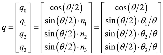 (9)
(9)
 (10)
(10)
The present study employs the algorithm proposed by Klumpp [12] and Spurrier [13] in order to avoid numerical singularity while extracting Euler parameters from a rotation tensor:
 (11)
(11)
where 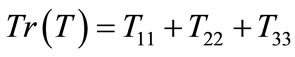 (12)
(12)
If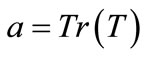 , each quaternion is obtained as follows
 (13)
(13)
 i = 1, 3 (14)
where i, j, k are the cyclic combination of 1, 2, 3.
If  but instead
 (15)
(15)
 (16)
(16)
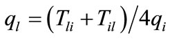 (17)
(17)
where, l = j, k Having obtained q0 to q3, for rotations of magnitude less than 180ْ, the rotation tensor can be obtained from (9) as follows
 (18)
(18)
where,  (19)
(19)
3. Determination of the Reference Coordinate System in a Nonlinear Space Frame Element
3.1. Overview
The present paper deals with a straight two-node space frame element based on the geometrically exact beam formulation. The original position vector of a node i has three components represented by a column vector 0i. Before any deformation works on an element, the nodal coordinate systems of two nodes are identical with the reference coordinate system 0C for the straight frame element (see Figure 1). There are numerous ways to establish this un-deformed reference coordinate system. Any procedure is available to choose these three element axes as long as the axes are perpendicular to each other. It is natural to set the first axis to coincide with an element chord and the others with the principal axes of the given section. Whatever coordinates are chosen, the orthogonality between three axes should always be satisfied in any deformed configurations as well as the un-deformed one.
Displacements applied on a node can be separated by translations ui and rotations θi. Note that the reference axes of these displacement vectors are the global coordinate system. The new position vector of the displaced node is decided by the translational displacement of a node, which is represented by 1i as follows.
 (20)
(20)
When the nodal rotations are invoked in a node i, the reference coordinate system 0C attached to a node is rotated to the deformed nodal coordinate iC by the rotation vector θi (see Figure 2). From the coordinate system rotation rule in (4), the deformed nodal coordinate system is given by
 (21)
(21)
The deformed nodal coordinates iC represent the applied

Figure 1. Coordinate system of a beam element in the un-deformed state configuration in space.

Figure 2. Deformed shape and nodal coordinate systems of a beam element in space.
rotations of a section in the node i. This rotation can be divided to two kinds of rotations; the rigid body rotation and the natural rotation. The rigid body rotations do not contribute any internal forces and deformations. Therefore, internal forces are only affected by the natural rotations, and the rigid body rotations can be neglected from the calculation of the total potential energy.
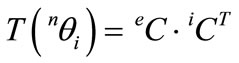
The translational displacements result in axial elongation or shortening of an element. They also contribute to the change of the reference coordinate system eC, which is determined from the nodal rotations iC. If a consistent reference coordinate system is assumed to be already determined by a proper method, the natural rotations nθi for a node i are obtained from vector multiplication with the consistent reference coordinates eC and the deformed nodal coordinates iC. By the definition of the natural deformation, the reference coordinate system is deformed by the natural rotation vector nθi to the corresponding reference axes of the nodal coordinates system. Therefore, according to (8), the natural rotation tensor is obtained:
 (22)
(22)
The rotation tensor T(nθ) results the natural rotation vector nθ according to the procedure given in Equations (11-19) to extract the rotation vector from the rotation tensor. The components of the rotation vectors nθi for a node i give the natural rotations on the node.
Choosing a consistent reference coordinate system is crucial for the performance and accuracy of the implementation of the geometrically exact beam formulation. Many researchers have investigated the procedures to establish a consistent reference coordinate system. The present paper presents two representative methods and introduces a new method: the ZTSC procedure.
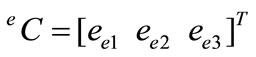
The reference coordinate system of a 3D beam element consists of three unit vectors, which represent each axis of the element (ee1, ee2 and ee3) and are perpendicular to each other (see Figure 3). The reference coordinate system eC can be expressed as a form of the rotation tensor as follows
 (23)
(23)
where the 1-axis unit vector, ee1, is determined straightforwardly by the deformed position vectors of two end nodes, i and j, as given in (24), because it should match with the direction of the chord of a member.
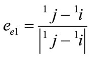 (24)
(24)
3.2. Determination of the 2-and 3-axes of the Reference Coordinate System
The decision of the 2- and 3-axes of a 3D beam element is not as definite as that of the 1-axis when large rotations and deformations are involved. In the un-deformed configuration, the 2- and 3-axes are unit vectors of the principal axes by which member sectional properties are defined. After deformation works on the element, they are distorted from the original reference coordinate system 0C. This paper focuses on how the principal or reference axes should be defined. Representative previous methods are briefly described in order to demonstrate the significance of the proposed method.
Yang and Kuo [8,9] developed a procedure to determine the reference coordinate system using vector projection to a given surface. The 1-axis, ee1 of the reference coordinate system is defined by (24), and the other 2- and 3-axes should exist on a plane 1S that is perpendicular to ee1 (see Figure 4). Thus, the 2- and 3-axes of the nodal coordinate system are projected to the plane 1S for each iand j-node. Then, its normalized projection vectors are obtained via (25). This method assumes that ee2 and ee3 are the mean vectors of the projection vectors. Consequently, the normalized mean vectors become (26)
 (25)
(25)
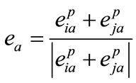 (26)
(26)
where p stands for projection to the perpendicular plane to the 1-axis 1S, a stands for the 2- and 3-axis of nodal coordinate system, and k stands for the two nodes i and j.
These averaged vectors do not guarantee that they are perpendicular to each other. This orthogonality of axes should always satisfy the definition of the Cartesian
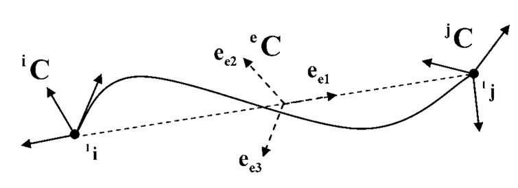
Figure 3. The reference coordinate system of a beam element in space.
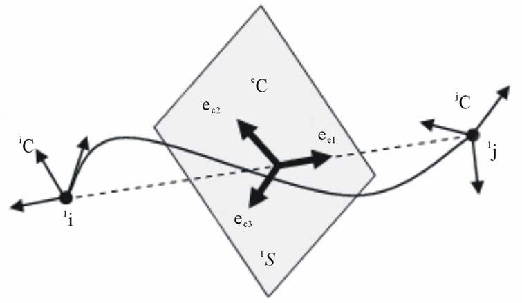
Figure 4. Kuo and Yang’s method to determine the reference coordinate system.
coordinate system and the the semi-tangential rules proposed by Argyris [10]. In order to establish the orthogonal axes system, further modifications are necessary (see Figure 5). Based on the property that the diagonals of a rhombus are perpendicular to each other and that they divide the interior angles of the rhombus equally, the normalized diagonals of the rhombus formed by the vectors e2 and e3 can be expressed as
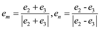 (27)
(27)
Rotating the unit vector em and en counterclockwise by 45 degrees, the 2- and 3-axes of the reference coordinate system are obtained as
 (28)
(28)
Although the application of the property of the rhombus is an intelligent decision and can be regarded as fair approach for moderate rotations, the physical meaning is nothing but an averaging process.
Crisfield [6,7] has also developed a procedure to determine the reference coordinate system. This method defined a rotation vector γ that rotates the i-nodal coordinate system, iC, to the j-nodal coordinate system, jC, as follows
 (29)
(29)
This approach assumes that the reference coordinate system is a rotated coordinate system from the i-node nodal coordinate system with half the angular rotation of γ (see Figure 6):
 (30)
(30)
Although the mean reference coordinate system eCm is based on a solid reasoning, the 1-axis em1 may not coincide with ee1 of (24). This means that the 2- and 3-axes do not exist on the plane 1S that is perpendicular to the 1-axis of the element. Therefore, the mean rotation tensor eCm needs to be revised based on the exact ee1 of (24) to obtain the remaining coordinates of the reference coordinate system ee2 and ee3 as follows
 (31)
(31)
While Kuo and Yang’s procedure does not meet the orthogonality between the 2- and 3-axes, and the Crisfield’s procedure does not satisfy between the 1-axis and the plane on the 2- and 3-axes. These two representative methods to determine the reference coordinate system both require revision, primarily because they chose the half value of the projection vector or the half of the rotation angle of the rotation tensor. These halves do not implicit a certain physical meaning but a revision to meet the orthogonality. The present paper will introduce a new
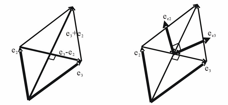
Figure 5. The rhombus procedure to revise the 2- and 3-axes of the reference coordinate system.

Figure 6. Crisfield’s method to determine the reference coordinate system.
method to determine the reference coordinate system that will not require any revision. In order to overcome the existing limitations in the determination of the reference coordinate system in the large rotation problem, it is necessary to involve one more condition.
The additional condition is the physical property of the natural torsion of beam elements, which is first introduced in the natural approach of Argyris et al. [14]. Kim et al. [15-17] and Hsiao et al. [18-21] also employed this condition to define the natural deformation. Let us define the natural torsions as nθi1 and nθj1 for each node, which is a rotation about the 1-axis of the reference coordinate system. In the natural deformation concept, these two torsional deformations nθi1 and nθj1 have to be same magnitude with opposite signs, as follows
ZTSC; (32)
(32)
This condition implies a physical condition that a section that does not twist always exists at a point between two nodes. In the present study, the authors suggest that this condition be called as the Zero Twist Section Condition (ZTSC).
Figure 7 presents a simple example to illustrate the concept of the ZTSC. Let us assume a straight circular bar with torsional displacements at both ends in order to neglect the effect of the warping torsion. If the left end rotates 10 degrees and the right end 20 degrees, the zero twisted section (ZTS) exists within a bar as shown in shaded section of Figure 7. This section experiences no torsional deformation but the rigid body torsion is 15 degrees. Then the natural torsion of an end is a relative rotation to the zero twist section, the natural torsion of left end becomes –5 degrees and right end +5 degrees. This example satisfies naturally the Zero Twist Section Condition (ZTSC). Even if compound rotations are induced, this condition should always be satisfied.
As mentioned before, earlier researchers have proposed various kinds of methods to determine the reference coordinate system on a space frame or beam element considering large rotations. However, most of them applied an averaging concept. Consequently, some special tactics are required in order to retain the orthogonality of the three axes of the reference coordinate system. If we adopt one more condition, that is ZTSC, we can decide a consistent reference coordinate system by means of a rational physical meaning without requiring any revision processes.
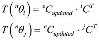
The proposed process requires iterations, which naturally reflects the nonlinear property of the finite rotations. As the first step of the ZTSC procedure, the initial coordinate system eCini that satisfies the orthogonality should be decided. The first row of the reference coordinate system eC must be the 1-axis, as given in (24). It is practical to use a procedure suggested by other researchers, such as that by Kuo and Yang or Crisfield, as an initial one. Whatever method is applied, in the initial coordinate system, the three axes must be orthogonal to one another and the first row should be the unit vector to the direction of the member chord, such as ee1, which can easily be obtained from the two nodal position vectors. From the nodal coordinate system iC or jC and the initial reference coordinate system eCini, we can obtain the rotation tensor of the natural rotation T(nθi) or T(nθj) according to (22) for each node:
 ,
, (33)
(33)
From the natural rotation tensor T(nθ), the natural rotation vector nθ of each node is extracted by the method proposed by Klumpp [12] and Spurrier [13] as described in (11-19). As a next step, convergence should be evaluated, and it is determined by whether or not the ZTSC is satisfied by means of the natural rotations nθi1 and nθj1. For a numerical implementation, a sufficiently small number ε for a convergence such as 1.0 × 10⁻⁵, is adopted:
ZTSC evaluation: (34)
(34)
where, ε is a sufficiently small number.
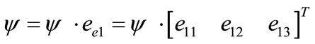
If the obtained natural rotations do not satisfy the ZTSC of (34), the reference coordinate system should be updated. Otherwise, the reference coordinate system and the natural rotations are successfully determined based on the ZTSC method. To update the existing reference coordinate system, the 2- and 3-axes of the reference coordinate system are rotated by ψ about 1-axis ee1. The rotation angle should apply the average value of the current natural torsion to each node, as given in (35). In other words, the updated rotation vector should have an angle of ψ and rotation axis of ee1. Therefore, the rotation vector to perform this updating rotation to the current reference coordinate system is given according to the definition of the rotation vector, as given in (36). The rotation tensor to update the current reference coordinate system can be obtained by the definition of the rotation tensor. The updated reference coordinate system can be expressed as (37). The newly updated reference coordinate system gives the new natural rotation tensors:
 (35)
(35)
 (36)
(36)
 (37)
(37)
 (38)
(38)
This process performs iterative calculations until the ZTSC convergence evaluation of (34) is satisfied. The complete process is shown in Figure 8. The ZTSC procedure concludes with consistent natural rotations and the reference coordinate system simultaneously, without any assumptions or a revision process.
3.3. Evaluation of Unbalanced Member Forces
In the nonlinear analysis of a structure, an iterative calculation is required, and it is very important that the member force is precisely calculated at the deformed configurations. In the iterative evaluation based on the geometrically exact beam formulation, total element forces are obtained from incremental or total internal forces. The natural rotations are obtained consistently from the ZTSC procedure. At the same time, the transformation matrix between the deformed reference and global coordinate system, that is the rotation tensor of the reference coordinate system, is also obtained according to the ZTSC procedure.
The internal forces are obtained from the element stiffness matrix tKe and the natural deformation Un in (39). This study applies the tangent stiffness matrix of Kim et al. [22] based on the geometrically exact beam formulation. Members forces are calculated from deformation according to force-displacement relationships given in (40).
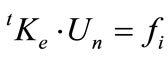 (39)
(39)
where 

 (40)
(40)
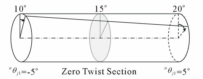
Figure 7. An example of a zero twist section.

Figure 8. Algorithm of the ZTSC procedure to determine the reference coordinate system and natural rotations.
where, ux, uy and uz are rigid body translations of the cross-section; f is a parameter defining the warping of the cross-section; f1, f2 and f3, are the axial and shear forces; m1 is the total twisting moment; m2 and m3 are the bending moment; and mR and mø are the restrained non-uniform torsional moment and the bimoment.
The total member force is evaluated by accumulating the incremental member forces at the global coordinate system. Therefore, the internal member force fi is transformed to the global member forces Fi and summarized for all elements in (41). The internal force vector Fi should be same as the external load b, if self equilibrium is satisfied. The difference between the internal forces and the external loads is the unbalanced member force vector Ф in (42).
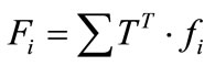 (41)
(41)
where 
 (42)
(42)
In a geometric nonlinear analysis, the unbalanced load is introduced as applied loads at the next iteration. The iteration procedure is performed until the convergence criterion is satisfied. In this study, the convergence criterion of the unbalanced load is introduced as the ratio of the 2nd-norm of the unbalanced load and the total applied load; it must be less than or equal to 1.0 × 10-N :
Convergence criterion:
 (43)
(43)
4. Numerical Examples of Large Rotations and Translations with Single Element Implementation
Examples of this section investigate a single space frame element involving an application of large amount of rotations and deformations in the three-dimensional space. The single element consists of two node beam element whose i-node is located at an origin and j-node is located at (1,0,0) so that the reference coordinates in the un-deformed configuration are equal to the global Cartesian coordinates.
In order to evaluate the numerical exactness of the methods, a new index is proposed: the ZTSC Index (ZI), which is defined as
 (44)
(44)
If ZI equals zero, it means that the ZTSC is completely satisfied. On the other hand, if ZI has a certain non-zero value, it represents that the calculated natural torsions do not satisfy the ZTSC value of the index. Therefore, as the absolute value of ZI is getting smaller, the calculation gives better results that are closer to satisfying the ZTSC.
It is obvious that the proposed ZTSC procedure always gives almost zero ZI, because it performs an iterative procedure until ZI becomes less than the convergence, which is given here as 1.0 × 10⁻⁵ in (34). On the other hand, the other methods such, as works done by Kuo and Yang or Crisfield, may not satisfy the ZTSC when large rotations and deformations are involved. The following examples will present the ZI of the other methods to demonstrate that these methods have drawbacks when large rotations are involved.
4.1 Case 1: Increasing Finite Rotations without Translation
Nodal rotations are applied at the j-node of an element with an angle of θj with respect to the three global coordinates in order to induce the spatial behavior, as shown in Figure 9. The three applied rotations vary from zero to ninety degrees at increments of one degree in (45). A section of the i-node does not rotate and maintains its un-deformed shape in the y-z plane.
Applied rotations for Case 1:
θj = (θj, θj, θj), 0˚ ≤ θj ≤ 90˚ (45)
When the rotational displacements are applied, the 1-axis of reference coordinate system of the element does not change at all because there are no applied translational displacements in the element. However, the 2- and 3-axes of the reference coordinates are distorted due to the action of the induced rotational displacements at the j-node. The analyses to determine the natural rotations are carried out according to three procedures: those proposed by Crisfield, Kuo and Yang, and ZTSC. The ZTSC procedure gives inherently an almost zero ZI. On the other hand, the other two procedures proposed by Kuo and Yang and Crisfield do not. The ZI for these two propositions are plotted in Figure 10 with respect to the imposed rotation angle θj. All of them give almost zero value until the rotation angle reaches up to 10 degrees. However, as the applied rotation is increasing, absolute ZI is gradually getting greater to negative value in case of the Crisfield’s procedure. This means that errors are accumulating in Crisfield’s method. Yang’s procedure generally achieves a better ZI value than Crisfield’s; however, a discontinuous point appears at 70 degrees due to the numerical instability.
The resulting natural torsions of the j-node are plotted in Figure 11. All analyses give almost the same results up to 20 degrees of applied rotation, although Crisfield’s result begins to deviate from the others at 20 degrees. It should be noted that Yang’s result has a discontinuous point around 70 degrees. When the rotations are greater than 70 degrees, the analysis gives zero torsion at the i-node and negative torsion at the j-node. This suggests that the resulting natural deformation from Yang’s procedure is not consistent after this discontinuous point. The flexural rotations with respect to the 2- and 3-axes exist only at the j-node, and Figure 12 shows the result of the rotations to 3-axis. The results also indicate that the rotations below 15 degrees are almost identical,
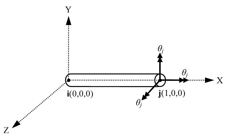
Figure 9. Case 1: Increasingly large rotations without translation.
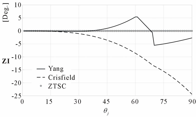
Figure 10. ZTSC Index of Case 1.
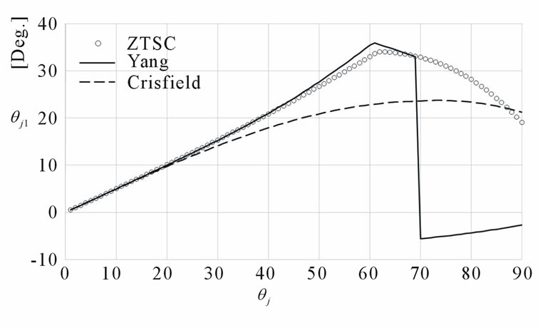
Figure 11. Natural torsions of the j-node for Case 1.
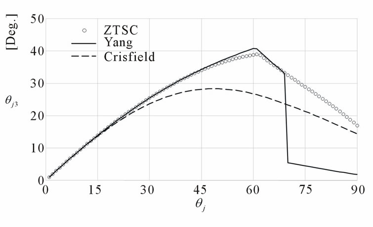
Figure 12. Flexural rotations of the j-node with respect to the 3-axis for Case 1.
although they begin to deviate as the applied rotations increase. In the case of Yang’s procedure, a discontinuous point appears at the same point as the natural torsion and the ZI. Crisfield’s procedure varies from the procedure of Yang or ZTSC beyond 20 degrees of rotation.
4.2. Case 2: Increasing Large Translations with Fixed Rotations
This example examines an element undergoing large translations accompanied by rigidly applied rotations. The original configuration of the element is the same as Case 1, and the section of the i-node is not rotated or translated. Consequently, the section at the i-node always remains in the same plane as the un-deformed configuretion. Case 2 involve a constant 10 degrees rotation at the section of the j-node with respect to each global axis. Additionally, the section of the j-node is rotated about the global Z axis, which results in translational displacements to the j-node. The rotation angle θT is applied as a translational displacement from 0 to 90 degrees. Meanwhile, two nodal sections of each node are not modified at all. Therefore, when the rotation angle reaches 90 degrees, the deformed shape of the element will look like an S-curve, as shown in Figure 13. The applied displacements and rotations are given:
Applied translations for Case 2:
ui = (0, 0, 0), uj = (cos θT, sin θT, 0), 0˚ ≤ θT ≤ 90˚ (46)
Applied rotations for Case 2:
θi = (0, 0, 0), θj = (10˚, 10˚, 10˚) (47)
The reference coordinate system of the example is identical with the global coordinate system in the un-deformed configuration. While the translational and rotational displacements are being applied at the j-node, the reference coordinate system changes continuously.
The ZI index results of the three analytical methods are plotted in Figure 14. The ZTSC procedure gives all zeros, which is inherent in the algorithm. Yang’s procedure provides more erroneous results, especially beyond 60 degrees translation; its maximum of absolute ZI reaches up to 7.5 degrees. In particular, when the applied translational angle is 90 degrees, Yang’s method is numerically unstable because the projection vector of the 2-axis at i-node, which is involved for the calculation of (26), becomes a zero vector so that the reference coordinate system cannot be obtained. This means that the Yang’s procedure is not applicable when the translation angle is exactly 90 degrees. On the other hand, Crisfield’s procedure achieves a small absolute ZI, which is about 0.4 degrees at most. It seems that Crisfield’s method gives relatively consistent results when large translations are applied.
The natural torsions for the i-node are plotted with respect to the rotated angle in Figure 15; the results of the j-node are shown the same manner as those of the i-node. The results are nearly identical between the three procedures until the translation angle reaches 15 degrees. As the rotated translation angle increases, the natural rotations from Crisfield’s procedure get larger. Based on this, it seems that Crisfield’s method may underestimate the torsional response for this case. On the other hand, Yang’s method gives inconsistent results at relatively large translations (greater than 65 degrees), which is expected based on its large ZI values at those angles.
The natural rotations about the 2-axis are given in Figure 16. The results are similar until the translation angle reaches 40 degrees. However, as the rotations get close to 90 degrees, the results spread apart. In the case of the 3-axis natural rotations, as shown in Figure 17, the results are similar until 70 degrees. They give better results than the other axis natural rotations. It is thought

Figure 13. Case 2: Increasingly large translations with fixed rotations.
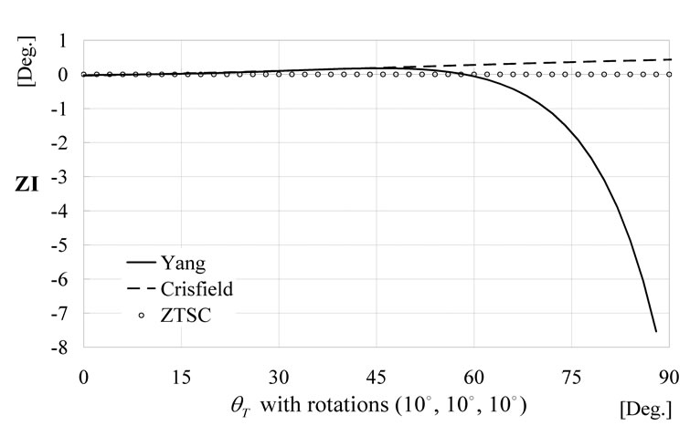
Figure 14. ZTSC index for case 2.
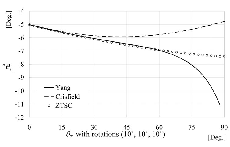
Figure 15. Natural torsions at the i-node for case 2.

Figure 16. Flexural rotations of the i-node with respect to the 2-axis for case 2.
that this superior agreement is caused by the fact that the transla tional rotation axis agrees with the 3-axis of the reference coordinate system.
From the above examples, it can be said that the natural rotations are fairly consistent across procedures when small rotations or translations are involved. However, as the rotations or translations increase, the resulting natural rotations can be distorted in violation of the ZTSC. The procedures other than ZTSC may underestimate the
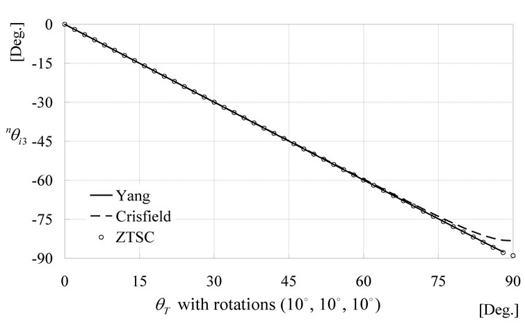
Figure 17. Flexural rotations of the i-node with respect to the 3-axis for Case 2.
structural response or cause numerical instability at finite rotations or in the translation problem. On the other hand, the ZTSC procedure always satisfies the ZTSC and calculates consistent natural rotations, even if large rotational or translational displacements are imposed.
5. Examples of Structural Analyses with the Geometrically Exact Beam Formulation
Various types of slender structures that undergo large displacements and deformations are introduced and analyzed by the finite element method implemented by the geometrically exact beam formulation. This study applies the implementation of the beam formulation developed by Kim et al. [22] in cooperation with the proposed ZTSC procedure. In the original research of Kim et al. [22], the reference coordinate system is determined from the rotation vector given in (48). This will be compared with current study for given examples.
 (48)
(48)
where,  is a torsional displacement of i-node;
  is a displacement to global n-axis; and
  is a deformed axial length of the element.
The arc-length method is used for the nonlinear analysis scheme. Each iteration procedure will be performed until the unbalanced load ratio is less than given convergence limit within the given maximum number of iterations. Unless it is converged, the load increment will be divided into a smaller one. Therefore, smaller number of load increments means better convergence. The given example structures are also analyzed by well-known commercial FE analysis program, ABAQUS with its own beam, solid and shell elements for comparison.
5.1. Cantilever 45-degree Bend Subject to Fixed End Vertical load
This example involves a genuine three-dimensional response that has been used by a number of authors [2,6, 23,24]. Figure 18 depicts the initial geometry and the induced vertical end load. The bend has a radius of 100 with a unit square cross-section. The material properties are E = 107 and G = 0.5 × 10⁷. The number of elements is chosen to be eight, which is the same as in previous studies, in order to compare the analysis results with former studies. The applied upward force is subjected from 0 to 1000. No units are involved in this problem.
ABAQUS is used to analyze the same model with beam (B31OS) and solid (C3D20R) elements. The beam element B31OS represents the 2-node open section space beam element. In this example, the same number of elements is examined. To compare the better result generated by a fine mesh model with the 20 node quadratic solid elements with reduced integration, C3D20R is also examined. 5008 solid elements with 28,235 nodes are used for the analysis. Figure 19 shows the refined finite element modeling with the solid elements.
Figure 20 shows the tip displacements as the applied load is increased up to 1000. The results from ABAQUS beam and solid element analyses are also given and the results from other authors [2,6,23,24] are depicted from their own papers for comparison. These analyses give almost the same tip displacements, while the solid element gives more axial displacements. These suggest that the developed procedure gives fine computational accuracy for the representative large displacement problem in space.
In order to evaluate the numerical efficiency of the developed ZTSC procedure, the numbers of load increments are compared to the analysis results followed by the procedure of Kim et al. [22]. Table 1 show the number of evaluated load increments for the non-linear analyses performed by the arc-length method. The first column “un-balanced load ratio” gives the convergence criterion from (43). In the general engineering structures

Table 1. Numbers of load increments for the cantilever with a 45 degree bend.
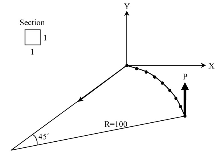
Figure 18. Initial geometry for a 45 degree bend.
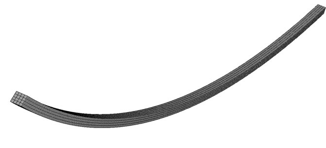
Figure 19. ABAQUS modeling of a 45 degree bend with solid elements.

Figure 20. Tip displacements of a 45 degree bend subjected to a vertical end load.
convergence of 10-3 is adequate, but the delicate structures may need smaller ones such as 10-4 or 10-5. The results tell that the developed ZTSC procedure reduces the load increments about half of the original one. This means that the ZTSC procedure provides a meaningful acceleration of the numerical efficiency of the analysis.
5.2. Mono-Symmetric Curved Cantilever under an Axial End Load
Figure 21 shows a curved cantilever subjected to an axial tip load and its mono-symmetric cross sectional geometry and material properties. The curved cantilever is modeled with 18 straight space beam elements, including a warping degree of freedom. The load is applied at the centroid of the section. In order to compare analysis results, two kinds of ABAQUS elements are analyzed. The first one is an open section beam element (B31OS) with the same number of elements. The second is a 6-node quadratic triangular thin shell element (STRI65) using five degrees of freedom per node. The shell model consists of 197 nodes and 81 elements as shown in Figure 22.
The critical buckling loads are obtained from the Eigen analysis given in Table 2, which demonstrates that the three models give almost the same results. Postbuckling behavior is analyzed until the applied load reaches up to 2.0. Figure 23 gives axial and lateral displacements of three analysis methods. The present method gives closer displacement curves to that of the ABAQUS shell element than that of the ABAQUS beam element. Numerical efficiency is also compared to the original one, according to the work of Kim et al. [22] without applying the ZTSC procedure, and required load increments are only 11% or less compared to the original one as given in Table 3. The required load increments for work by Kim et al. are getting larger than that of the
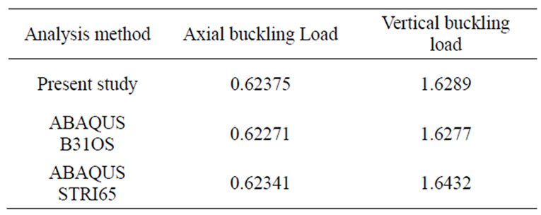
Table 2. Critical buckling loads of the curved cantilever.
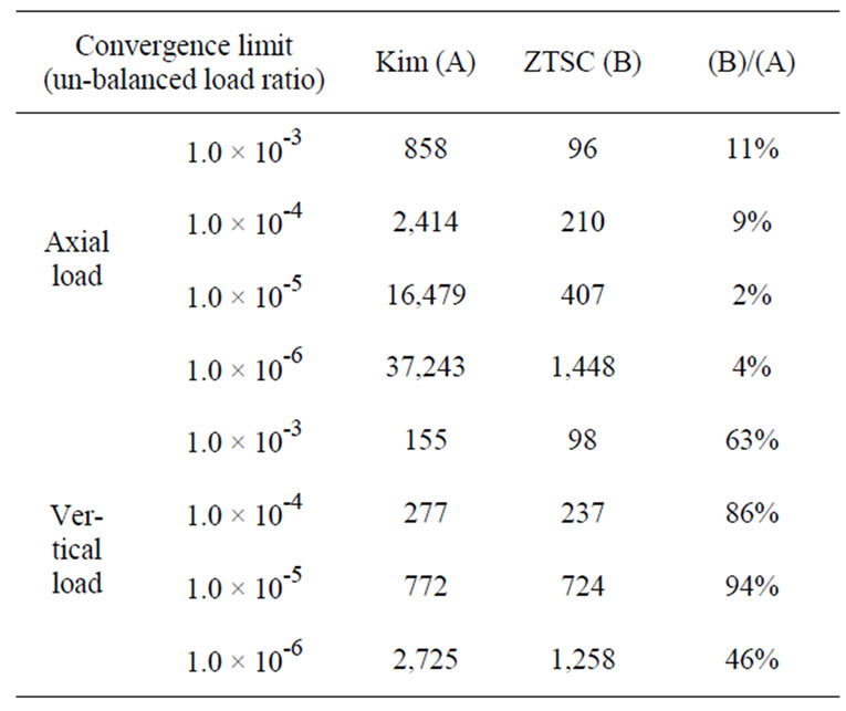
Table 3. Numbers of load increments of the curved cantilever.
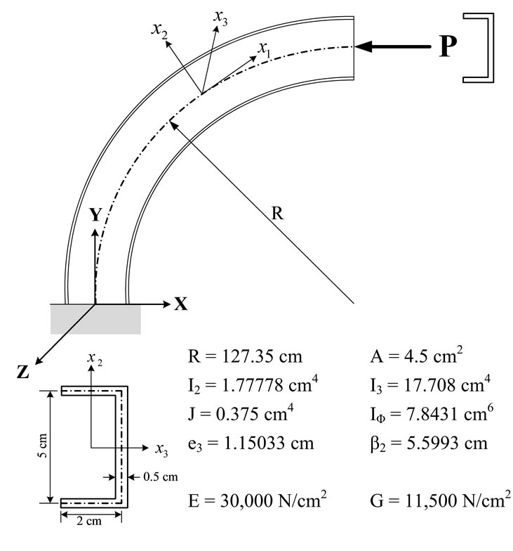
Figure 21. Initial geometry of a mono-symmetric curved cantilever under an axial end load.
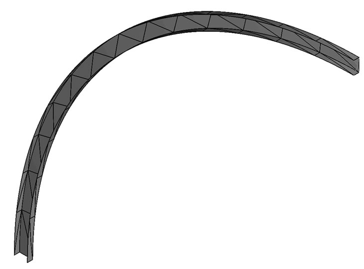
Figure 22. ABAQUS modeling of a mono-symmetric curved cantilever with shell elements.

Figure 23. Tip displacements of a mono-symmetric curved cantilever under an axial end load.
ZTSC as the convergence criterion is getting severer. These results suggest that the ZTSC procedure can significantly improve numerical efficiency, especially when superior numerical exactness is required.
5.3. Mono-Symmetric Curved Cantilever under a Vertical End Load
Analyses are performed to the same structure of the above section with an upward vertical end load in the Y-direction, instead of an axial load, is applied at the centroid point of the end tip. The buckling loads are obtained given in Table 2 from the eigen-value analysis, which shows good agreement between the analyses. In the post-buckling analysis, the present method gives similar results to the others, as shown in Figure 24. The required load increments are also given in Table 3. The present method can also increase the numerical efficiency also in the vertical load case.
5.4. Non-Symmetric Cantilever under an Axial End Load
Figure 25 shows a cantilever beam subject to an axial load at a centroid point of the end tip. The material and geometric properties of its non-symmetric open channel section are also given in Figure 25. The cantilever is modeled with 10 straight beam elements including a warping degree of freedom. The local 2- and 3-axes at the un-deformed state are rotated with angle θ, as shown in Figure 25, because this section is non-symmetric in both directions. This cantilever structure is analyzed with the present study and the ABAQUS beam (B31OS) and shell (STRI65) elements. The shell model consists of 106 nodes and 42 shell elements, as shown in Figure 26.
The eigen-value analysis gives the critical buckling loads as given in Table 4. Figure 27 shows the tip displacement results from the three analyses. The ABAQUS beam element gives almost the same results as the analysis results done by the ZTSC procedure of this study, although the shell element gives smaller axial displacements. The reason for this difference is that the beam assumptions are not valid for this extremely large deformation case, considering that the total length of the member is only 200 cm. Load increments are given in Table 5, which indicates that the numbers of load

Table 4. Critical axial buckling load of the cantilever

Table 5. Numbers of load increments of the cantilever under an axial end load.
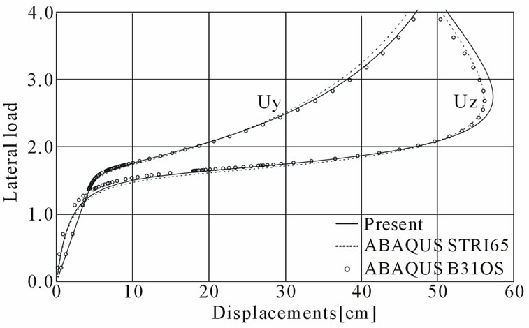
Figure 24. Tip displacements of a mono-symmetric curved cantilever under a vertical end load.
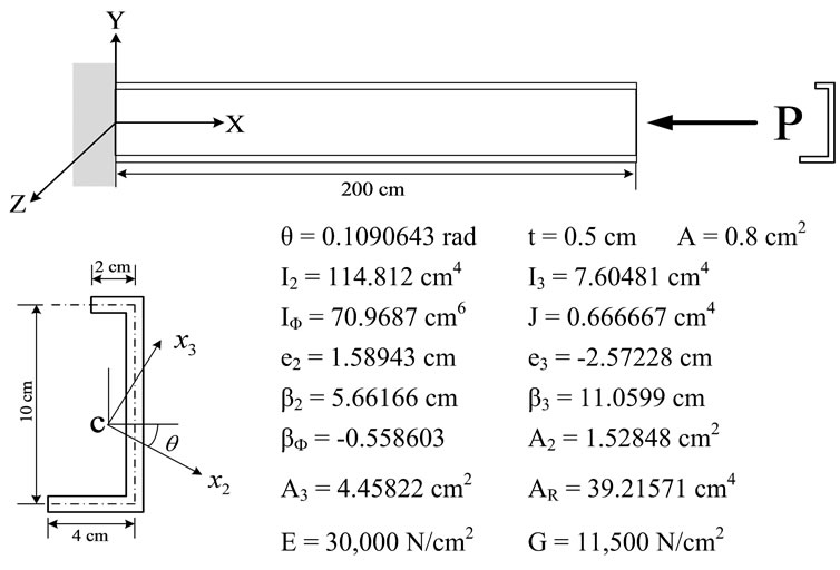
Figure 25. Initial geometry of a non-symmetric cantilever under an axial end load.

Figure 26. ABAQUS modeling of a non-symmetric cantilever with shell elements.
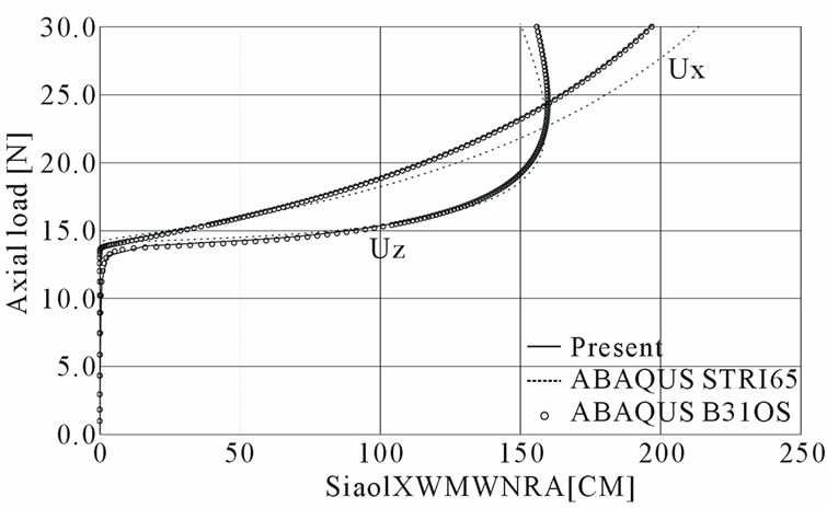
Figure 27. Tip displacements of a non-symmetric cantilever under an axial end load.
increments are similar when the convergence un-balanced load ratios are between 10-3 and 10-4. However, when the convergence condition is very tight, in the range of 10-5 to 10-6, the developed ZTSC procedure gives better numerical efficiency.
6. Conclusions
The present paper has described a procedure to determine the reference coordinate system for the geometrically exact beam formulation in three-dimensional space under large rotations and deformations. A new concept, the Zero Twist Section Condition (ZTSC) is introduced to decide the physically meaningful reference coordinate system with consistency, even under a combination of large spatial rotations and deformations. Since the previous studies are not based on physical meaning, they require revision processes. The concept of the ZTSC is that the twisted natural torsions at the two end nodes of a beam element always have to be the same magnitude and opposite signs. Based on this condition, an iterative procedure is developed to determine the reference coordinate system: the ZTSC procedure.
Two other previous methods proposed by Yang and Crisfield to calculate natural rotations for finite nodal rotations or translations are compared to ZTSC procedure. The results show that the other procedure may induce results which do not satisfy the definition of the Cartesian coordinate system, especially when large rotations or translations are imposed. Although these large rotation and translation are rather difficult to encounter for a practical nonlinear analysis, it is meaningful that this study suggests a more accurate procedure than previous ones for a combination of exceedingly large rotations.
The developed ZTSC procedure is implemented in the geometrically exact formulation developed by Kim et al. [22], whose numerical performance is compared with load increments in the arc-length procedure to follow the post-buckling behavior of the structures. The analysis demonstrates fairly good agreement with the other analyses with smaller load increments, which indicates that the developed procedure can accelerate the numerical process of the geometrically exact beam formulation. As a result, a new method is developed to determine the reference coordinates for a beam element involving very large rotations and deformation in three-dimensional space. It is proved that the developed ZTSC procedure is sufficiently applicable to the large rotation and deformation problem in cooperation with the geometrically exact beam formulation.
7. Acknowledgments
This work was a part of a research project supported by the Korea Ministry of Construction & Transportation (MOCT) through the Korea Bridge Design & Engineering Research Center at Seoul National University. It was also supported by the Korea Research Foundation Grant funded by the Korean Government (KRF-2008-357- D00261). The authors wish to express their gratitude for the financial support. In addition, the author wants to express gratitude to professor Hassan H. Abbas in Auburn University for his kind help and support.
8. REFERENCES
- E. Reissner, “On One-Dimensional Finite-Strain Beam Theory: The Plane Problem,” Journal of Applied Mathematics and Physics (ZAMP), Vol. 23, No. 5, 1972, pp. 795-804. doi:10.1007/BF01602645
- J. C. Simo and L. Vu-Quoc, “A Three-Dimensional Finite-Strain Rod Model. Part II: Computational Aspects,” Computer Methods in Applied Mechanics and Engineering, Vol. 58, No. 1, 1986, pp. 79-116. doi:10.1016/0045- 7825(86)90079-4
- A. A. Shabana and R. Y. Yakoub, “Three Dimensional Absolute Nodal Coordinate Formulation for Beam Elements: Theory,” Journal of Mechanical Design, Vol. 123, No. 4, 2001, pp. 606-613. doi:10.1115/1.1410100
- R. Y. Yakoub and A. A. Shabana, “Three Dimensional Absolute Nodal Coordinate Formulation for Beam Elements: Implementation and Applications,” Journal of Mechanical Design, Vol. 123, No. 4, 2001, pp. 614-621. doi:10.1115/1.1410099
- I. Romero, “A Comparison of Finite Elements for Nonlinear Beams: The Absolute Nodal Coordinate and Geometrically Exact Formulations,” Multibody System Dynamics, Vol. 20, No. 1, 2008, pp. 51-68. doi:10.1007/ s11044-008-9105-7
- M. A. Crisfield, “A Consistent Co-Rotational Formulation for Non-Linear, Three-Dimensional, Beam-Elements,” Computer Methods in Applied Mechanics and Engineering, Vol. 81, No. 2, 1990, pp. 131-150. doi:10. 1016/0045-7825(90)90106-V
- M. A. Crisfield, “Non-linear Finite Element Analysis of Solids and Structures,” John Wiley & Sons, Hoboken, 1997.
- S. R. Kuo, Y. B. Yang and J. H. Chou, “Nonlinear Analysis of Space Frames with Finite Rotations,” Journal of Structural Engineering, Vol. 119, No. 1, 1993, pp. 1-15. doi:10.1061/(ASCE)0733-9445(1993)119:1(1)
- Y. B. Yang and S. R. Kuo, “Thoery & Analysis of Nonlinear Framed Structures,” Prentice Hall, Upper Saddle River, 1994.
- J. Argyris, “An Excursion into Large Rotations,” Computer Methods in Applied Mechanics and Engineering, Vol. 32, No. 1-3, 1982, pp. 85-155. doi:10.1016/0045- 7825(82)90069-X
- M. A. Crisfield, “Non-linear Finite Element Analysis of Solids and Structures,” John Wiley & Sons, Hoboken, 1991.
- A. R. Klumpp, “Singularity-Free Extraction of a Quaternion from a Direction-Cosine Matrix,” Journal of Spacecraft and Rockets, Vol. 13, No. 2, 1976, pp. 754-755. doi:10.2514/3.27947
- R. A. Spurrier, “Comment on ‘Singularity-free Extraction of a Quaternion from a Direction-Cosine Matrix’,” Journal of Spacecraft and Rockets, Vol. 15, No. 4, 1978, pp. 255-255. doi:10.2514/3.57311
- J. H. Argyris, et al., “Finite Element Method: The Natural Approach,” Computer Methods in Applied Mechanics and Engineering, Vol. 17-18, 1979, pp. 1-106. doi:10. 1016/0045-7825(79)90083-5
- M. Y. Kim, S. P. Chang and S. B. Kim, “Spatial Postbuckling Analysis of Nonsymmetric Thin-Walled Frames II: Geometrically Nonlinear FE Procedures,” Journal of Engineering Mechanics, Vol. 127, No. 8, 2001, pp. 779- 790. doi:10.1061/(ASCE)0733-9399(2001)127:8(779)
- M. Y. Kim, S. P. Chang and H. G. Park, “Spatial Postbuckling Analysis of Nonsymmetric Thin-Walled Frames. I: Theoretical Considerations Based on Semitangential Property,” Journal of Engineering Mechanics, Vol. 128, No. 8, 2001, pp. 769-778. doi:10.1061/(ASCE)0733-399- (2001)127:8(769)
- S. B. Kim and M. Y. Kim, “Improved Formulation for Spatial Stability and Free Vibration of Thin-Walled Tapered Beams and Space Frames,” Engineering Structures, Vol. 22, No. 5, 2000, pp. 446-458. doi:10.1016/S0141- 0296(98)00140-0
- H. H. Chen, W. Y. Lin and K. M. Hsiao, “Co-Rotational Finite Element Formulation for Thin-Walled Beams with Generic Open Section,” Computer Methods in Applied Mechanics and Engineering, Vol. 195, No. 19-22, 2006, pp. 2334-2370. doi:10.1016/j.cma.2005.05.011
- K. M. Hsiao and W. Y. Lin, “A Co-Rotational Finite Element Formulation for Buckling and Postbuckling Analyses of Spatial Beams,” Computer Methods in Applied Mechanics and Engineering, Vol. 188, No. 1-3, 2000, pp. 567-594. doi:10.1016/S0045-7825(99)00284-4
- W. Y. Lin and K. M. Hsiao, “Co-Rotational Formulation for Geometric Nonlinear Analysis of Doubly Symmetric Thin-Walled Beams,” Computer Methods in Applied Mechanics and Engineering, Vol. 190, No. 45, 2001, pp. 6023-6052. doi:10.1016/S0045-7825(01)00212-2
- K. M. Hsiao and W. Y. Lin, “A Co-Rotational Formulation for Thin-Walled Beams with Monosymmetric Open Section,” Computer Methods in Applied Mechanics and Engineering, Vol. 190, No. 8-10, 2000, pp. 1163-1185. doi:10.1016/S0045-7825(99)00471-5
- M. Y. Kim, N. I. Kim and H. T. Yun, “Exact Dynamic and Static Stiffness Matrices of Shear Deformable Thin-Walled Beam-Columns,” Journal of Sound and Vibration, Vol. 267, No. 1, 2003, pp. 29-55. doi:10.1016/ S0022-460X(02)01410-4
- K.-J. Bathe and S. Bolourchi, “Large Displacement Analysis of Three-Dimensional Beam Structures,” International Journal for Numerical Methods in Engineering, Vol. 14, No. 7, 1979, pp. 961-986. doi:10.1002/nme.162 0140703
- A. Cardona and M. Geradin, “A Beam Finite Element Non-Linear Theory with Finite Rotations,” International Journal for Numerical Methods in Engineering, Vol. 26. No. 11, 1988, pp. 2403-2438. doi:10.1002/nme.16202611 05