Journal of Modern Physics
Vol.4 No.5(2013), Article ID:31409,11 pages DOI:10.4236/jmp.2013.45079
Reverse Engineering Approach to Quantum Electrodynamics*
Geretsried, Germany
Email: wsmilga@compuserve.com
Copyright © 2013 Walter Smilga. This is an open access article distributed under the Creative Commons Attribution License, which permits unrestricted use, distribution, and reproduction in any medium, provided the original work is properly cited.
Received February 18, 2013; revised March 21, 2013; accepted April 19, 2013
Keywords: Quantum Electrodynamics; Fine-Structure Constant; Entanglement; Gauge Invariance; Reverse Engineering
ABSTRACT
The S matrix of e-e scattering has the structure of a projection operator that projects incoming separable product states onto entangled two-electron states. In this projection operator the empirical value of the fine-structure constant α acts as a normalization factor. When the structure of the two-particle state space is known, a theoretical value of the normalization factor can be calculated. For an irreducible two-particle representation of the Poincaré group, the calculated normalization factor matches Wyler’s semi-empirical formula for the fine-structure constant α. The empirical value of α, therefore, provides experimental evidence that the state space of two interacting electrons belongs to an irreducible two-particle representation of the Poincaré group.
1. Introduction
The development of quantum electrodynamics (QED) belongs to the greatest successes of theoretical physics. Provided that a sufficient number of terms of the perturbation series are included, the results of QED agree with the experimental data to any required degree of precision. This is a strong support for the correctness of the perturbation algorithm of QED. Nevertheless, we are far from completely understanding this algorithm. Although the success of QED has widely been considered as a confirmation of the concept of interacting quantum fields, i.e., of the electron field’s interacting with the photon field, theoretical considerations (e.g., Haag’s Theorem [2]) call into doubt that QED is really a quantum field theory of interacting fields. Aside from this open question of the compatibility of QED with the concepts of quantum field theory, notorious divergences plague the users of the algorithm. These divergences can be removed by renormalization, but their mere existence makes it difficult to really understand the perturbation algorithm. This does not prevent the majority of practitioners of QED from successfully using the perturbation algorithm, following the famous slogan: “Shut up and calculate” [3].
A similar situation is often encountered in software engineering, when a software program is available only as a (machine readable) object program, but not as (human readable) source code. Here, such situations are successfully handled by means of “reverse engineering” [4]. From Wikipedia [5]: “Reverse engineering is the process of discovering the technological principles of a device, object, or system through analysis of its structure, function, and operation.”
The term “reverse engineering” originally described the (sometimes illegal) use of mechanical engineering to analyze competitor’s products, when the original blue prints, for understandable reasons, were not available. Nowadays, reverse engineering is well-known in software engineering as a powerful, though sometimes cumbersome, method for reconstructing the original source code of a program by decompiling or disassembling the binary machine code when the source code is not available— whether it has been lost or whether it has not been made available by the original manufacturer.
When we buy a software product, we usually have to sign a licensing agreement similar to: “The use of the software is subject to the following restrictions: You are prohibited from decompiling, reverse engineering, or disassembling the software, or otherwise attempting to derive their source code.” In QED we are in the advantageous position that its perturbation algorithm is “public domain”, although we are not sure whether or not we are in the possession of the correct and complete “source code”. In any case, there is no licensing agreement that can prevent us from reconstructing the “source code” by reverse engineering. In view of six decades of “Shut up and calculate”, at least an attempt is long overdue.
In line with the approach used in software engineering, we will isolate the basic building blocks of the perturbation algorithm, and find each one’s mathematical functionality. Then we will put these building blocks together, to find their combined functionality. If carefully done, this will result in a consistent description of the perturbation algorithm, which can be regarded as the “source code” behind the algorithm. This description may then serve as a basis for a physical interpretation. It should not come as a surprise, however, if this interpretation turns out to not reproduce the physical concepts that historically led to the design of the perturbation algorithm.
Reverse engineering is usually followed by re-engineering the object under study, with the goal of improving or extending its functionality. The present paper is limited to the reverse engineering phase, and we will take strict care not to change the perturbation algorithm.
2. A Short Review of Quantum Electrodynamics
The following is a short overview of QED, as formulated by Feynman in his seminal papers of 1949/1950 [6-8].
QED uses a perturbation approach to the S matrix, which, for an electromagnetic scattering process, delivers the transition probabilities between the incoming and outgoing two-particle states. The incoming and outgoing states are described by states in Fock space. These states are constructed through repeated application of “creation” operators to a “vacuum” state. A particle in a Fock state can be annihilated through a corresponding “annihilation” operator. Creation and annihilation operators satisfy certain commutation or anticommutation rules, which ensure that the generated multi-particle states have the correct symmetry of either Fermi—Dirac statistics (electrons) or Bose—Einstein statistics (photons). Multiparticle states are first generated as pure product states. They are used to describe the “incoming” and “outgoing” states. Because these states are separable, there are no correlations between the individual particle states other than by the mentioned statistics, so that the incoming and outgoing states describe “free” particles. Linear combinations of separable product states, which in general will not be separable but entangled, then make up a full product state space, corresponding to a product representation of the Poincaré group.
The idea behind the concept of the S matrix is that without knowing exactly what happens in the “interaction region”, we should formulate a quantum mechanical scattering theory on the basis of the incoming and outgoing states, because only these states are directly accessible to the experimenter [9]. But since the incoming and outgoing states describe non-interacting particles, a heuristic “interaction term” is needed, to describe, at least in a phenomenological form, the process inside the interaction region. Since it seems reasonable that the interaction process is uniquely determined by incoming and outgoing states, it has been tried to construct interaction terms from creation and annihilation operators of the incoming and outgoing states. Relativistic (Poincaré) invariance greatly restricts the structure of such terms. It turns out that with the additional requirement of gauge invariance (of second kind), the interaction term
 (1)
(1)
is uniquely determined, up to a constant factor e. The factor e, the electromagnetic coupling constant, has been determined experimentally. Its square is the electromagnetic fine-structure constant ![]() (with the convention
(with the convention ). The field operators
  and
and  are operator-valued distributions.
 and
and  are field operators of the electron— positron field (cf. e.g. Scharf [10])
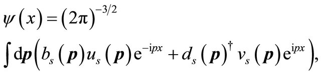 (2)
(2)
 is the Dirac adjoint operator,
  are the Dirac matrices, and
  means Hermitian adjoint.
  and
and  are solutions of the Dirac equation of, respectively, positive and negative energy.
 is the field operator of the electromagnetic field
 (3)
(3)
(ignoring the fact that  is usually defined in a slightly different way to ensure manifest Lorentz covariance).
The creation operator bs(p)† creates from the “vacuum state”  an electron state with momentum p and spin s,
 . The Hermitian adjoint operator
 is the corresponding annihilation operator; for the vacuum state
  holds.
  are the respective operators for positrons.
  create and annihilate a photon with momentum
![]() . We have the anticommutation rules
. We have the anticommutation rules
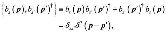 (4)
(4)
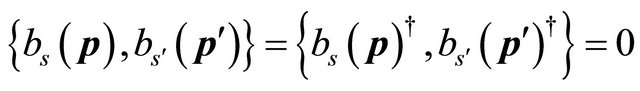 (5)
(5)
—analogous rules apply to —and the commutation rules
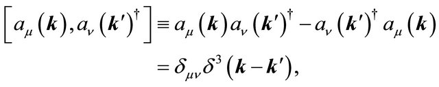 (6)
(6)
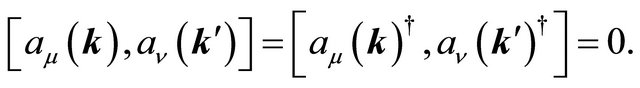 (7)
(7)
The lack of precise information about the “physical” processes inside the interaction region, and the association of the terms “creation” and “annihilation” with real dynamic processes, has led to our present picture of QED: a highly dynamic, not to say chaotic, interplay of particles, continuously created from the vacuum, annihilated just a short time later, only controlled by some conserved quantum numbers, such as charge and lepton number.
3. The S Matrix of (Elastic) Electron—Electron Scattering
The perturbation approach to QED uses the interaction term (1) as a “perturbation” to the “free” theory and expands the S matrix into a series of increasing orders in . The first order contribution is obtained from the twopoint distribution built from an iteration of the interaction term,
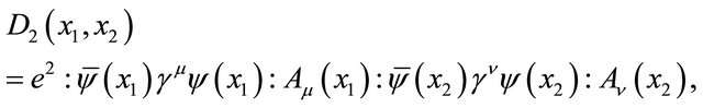
(8)
where the colons “![]() “ mean “normal ordering” (cf. e.g. Scharf [10]). Higher orders are constructed by iterating this first order contribution.
“ mean “normal ordering” (cf. e.g. Scharf [10]). Higher orders are constructed by iterating this first order contribution.
After inserting the explicit form of the field operators (2) and (3) into the two-point distribution (8), the corresponding first-order S matrix,
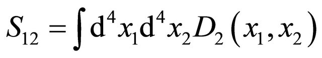 (9)
(9)
can be evaluated. By combining the phase factors of the field operators (2) and (3) with the integrations in Equation (9), we can construct ![]() functions of the form
functions of the form
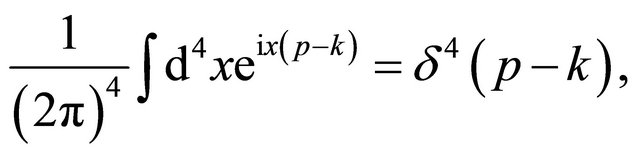 (10)
(10)
which can be used to rearrange the momenta. As an intermediate result, we obtain several terms of the structure (all c-numbers are replaced by “ “)
“)
 (11)
(11)
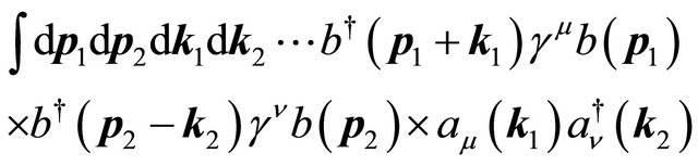
Contraction (permutation) of the photon operators results in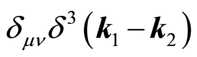 . By integrating over
 , we obtain

(12)
Although this term contains only electron operators, its familiar interpretation is this: a gauge particle (the photon) with momentum ![]() is emitted from particle 2 and absorbed by particle 1, causing transitions from
is emitted from particle 2 and absorbed by particle 1, causing transitions from  to
to  and from
  to
to .
.
Mathematically, this term has a more prosaic interpretation: The S matrix, when evaluated between incoming and outgoing states, describes a transition from an incoming two-particle product state to an entangled twoparticle state and then back to an outgoing product state. The entanglement is caused by the integration over![]() , whereas the integration over
, whereas the integration over  and
and  means an integration over a complete set of base states of the product state space.
4. Two-Particle State Space and the Fine-Structure Constant
The functionality of the (first order) S matrix, as just described, closely resembles the operation of a projection operator onto an intermediate two-particle subspace of the product state space. In the following, this will be further substantiated.
Observe that the range of integration over  and
and  is automatically restricted to the subspace of the parameter space with a total momentum P, which equals the sum of the momenta of the incoming particles. This means, the total momentum is conserved at each “vertex”. This property is preserved in higher orders of the perturbation series, because these are obtained by iterating the first order S matrix. The entangled intermediate states, therefore, belong to a subspace of the product state space, characterized by a constant total momentum P. The fact that the states are entangled indicates a further restriction. Since the perturbation algorithm is formulated in a covariant way, we can assume that this subspace is part of a relativistically invariant subspace, characterized by P2 = some constant. Let
  be a manifold that parametrizes this subspace and let
  denote the volume of
 .
.
The states of this invariant subspace can be represented by linear combinations of base states , generated from the vacuum by two creation operators
 (13)
(13)
with . The corresponding “bra” states are
 (14)
(14)
Observe, however, that by the anticommutation rule (4), these states are still normalized to the volume of the full product state space. Since a correct normalization is a precondition for the calculation of transition probabilities, the normalization has to be adjusted to the volume of this subspace.
Let us, for a while, forget that the volumes of the parameter spaces considered so far are infinite. Then the correct normalization factor of a base state should be determined by the volume , calculated from an embedding of
  into the parameter space
  of the product state space, resulting in a factor
![]() .
.
When these states or their creation/annihilation operators, respectively, are used to construct a projection operator such as integral (12), then the normalization factor enters as .
.
Since the goal of reverse engineering is a consistent mathematical description, we have to prove that this projection operator is in fact used in a way that is mathematically consistent with the requirements of a correct normalization. Therefore our next step is, in general terms, to calculate  and then compare this value with a corresponding normalization factor that is extracted from the perturbation algorithm.
 can be determined independently from the evaluation of integral (12) by calculating the Lebesgue integral over the manifold
 . With the metric induced on
  by its embedding into
 , the Lebesgue integral can formally be written as
 (15)
(15)
where  is the Lebesgue measure on
 .
.
Let us, after the calculation of , replace the Lebesgue measure by
 (16)
(16)
and then convert  into a normalized Cartesian volume element
 (17)
(17)
where
 (18)
(18)
Besides the factor ,
,  contains an additional factor due to the conversion of the non-Cartesian
 into the Cartesian volume element
 .
.
Then integral (15) takes on the form
 (19)
(19)
The way in which  is presented in Equation (18) indicates that only the ratio of the infinitesimal volume element
  to the infinitesimal volume element
 needs to be determined. Therefore, we are free to map both parameter spaces onto, for example, a finite (bounded) parameter space, before we perform the calculation of
 , provided that this mapping does not change the ratio of the infinitesimal volume elements.
Based on Equation (18),  can be understood as a measure for the number of irreducible two-particle states contained in the infinitesimal volume element
  of the product representation, or as a weight factor that weights the contribution of the subspace to the full product state space. In the following, we will therefore refer to
  as a “weight factor”. Because of the relativistic covariance of the S matrix,
  does not depend on the frame of reference.
After having calculated , we will try to insert
  into integral (12), to give this expression the consistent structure of a projection operator. However, when inserting
 , we notice that in the same position, the square of the empirical electromagnetic coupling constant e, i.e., the fine-structure constant
![]() , is also inserted “by hand” to reproduce the experimental data. Hence, after having inserted the empirical value of
, is also inserted “by hand” to reproduce the experimental data. Hence, after having inserted the empirical value of![]() , we cannot, in addition, insert the calculated weight factor without affecting the calculated transition amplitudes. This conflict is resolved if
, we cannot, in addition, insert the calculated weight factor without affecting the calculated transition amplitudes. This conflict is resolved if ![]() and the weight factor
and the weight factor  associated with the two-electron state space are one and the same.
Under this premise, the calculation of  takes on an entirely new significance: We should be able to identify the correct two-particle state space of e-e scattering by selecting a promising state space, calculating the numerical value of
 , and comparing it to the experimentally determined value of
![]() . If we find that the two coincide, i.e.,
. If we find that the two coincide, i.e.,
 (20)
(20)
we can consider this as experimental evidence that we have found the correct two-particle state space.
Now let us see how this idea can be put into practice.
5. Irreducible Two-Particle Representation
The smallest relativistic invariant subspace of the product state space is the space of an irreducible two-particle representation of the Poincaré group. It represents the quantum mechanically correct description of an isolated two-particle system.
Let  and
and  be the 4-momenta of two electrons. They satisfy the mass shell relations
 (21)
(21)
where ![]() is the mass of the electron. We also introduce the total and relative momentum by
is the mass of the electron. We also introduce the total and relative momentum by
 (22)
(22)
By this definition,  and
and  satisfy
 (23)
(23)
Based on relation (23), any two-particle state (reducible or irreducible) can be described by a total momentum P and a spacelike momentum q, perpendicular to the timelike vector P. Perpendicular to a timelike vector means that q is allowed to rotate by the action of a  subgroup of the Lorentz group.
For an irreducible two-particle representation, the relation
 (24)
(24)
(mass hyperboloid) holds. The “mass” M corresponds to the value of one of two Casimir operators (see below) that characterize an irreducible two-particle representation of the Poincaré group. From Equation (24) we obtain
 (25)
(25)
Equations (24) and (25) can be combined to
 (26)
(26)
Equation (25) can be rewritten as
 (27)
(27)
or
 (28)
(28)
Equations (27) and (28) correlate the particle momenta by fixing the angle between them and with respect to P. Provided that P is not in its rest frame, rotations with rotational axis P preserve these angles. Since these rotations leave P invariant, they can be related to a rotational degree of freedom that is independent of the kinematics of P. These rotations are described by an action of , acting synchronously on
  and
and  and therefore also on the relative momentum
 . For P in its rest frame,
  , the orientation of the axis of the
  rotations is undetermined, which allows for any axis perpendicular to
 .
.
Within an irreducible representation, the relative momentum q can therefore be understood as a (2 + 1)- dimensional vector embedded in![]() .
.
The action of  on P, together with the action of
  on q, generates the manifold
 , which parametrizes the state space of an irreducible two-particle representation labeled by M. The
  moves within
  as P moves through the hyperboloid (24). The manifold
  can therefore be described as a circle bundle over a hyperboloid.
6. Calculation of the Weight Factor
To determine the numerical value of  for an irreducible two-particle representation, we will evaluate the Lebesgue integral (19) “from scratch”, using a bounded parametrization of
 , to take advantage of the finite environment.
Due to the hyperbolic/circular structure of , we can expect that
  will contain contributions of volumes of circular or hyperbolic shapes. This should remind us of a finding of the Swiss mathematician Armand Wyler, who in 1971 published a formula that approximates the electromagnetic fine-structure constant
 ![]() to a high degree of precision [11]. When Wyler found his formula, his favorite subject was: “the various components of the boundaries of complex domains associated with Lie groups” [12]. He observed that an expression, derived from the volumes of some homogeneous domains, related to Maxwell’s equations, delivered the numerical value of the fine-structure constant. He published his finding in the hope that “if he piqued the interest of the physics community, there might be more study of his favorite subject” [12]. Unfortunately, the physics community neither understood his intention nor his mathematics. Since Wyler was not able to put his observation into a convincing physical context, his paper was criticized [13] and, in the following decades, it was considered as fruitless numerology [14].
to a high degree of precision [11]. When Wyler found his formula, his favorite subject was: “the various components of the boundaries of complex domains associated with Lie groups” [12]. He observed that an expression, derived from the volumes of some homogeneous domains, related to Maxwell’s equations, delivered the numerical value of the fine-structure constant. He published his finding in the hope that “if he piqued the interest of the physics community, there might be more study of his favorite subject” [12]. Unfortunately, the physics community neither understood his intention nor his mathematics. Since Wyler was not able to put his observation into a convincing physical context, his paper was criticized [13] and, in the following decades, it was considered as fruitless numerology [14].
Our calculation of  will show that Wyler was perfectly right when he proposed his formula. Just like Wyler, we will make use of some elements of the mathematical theory of symmetric homogeneous (bounded) domains (cf. e.g. [15]).
We can understand a symmetric homogeneous domain as an abstract parameter space on which a Lie group acts transitively as a symmetry group. “Transitively” means that all points of the homogeneous domain can be obtained from any given point by an action of the symmetry group. Accordingly, a quantum mechanical state space that has been parametrized by a symmetric homogeneous domain can be generated from a given point of the domain by the simultaneous application of the full symmetry group to both the parameter space and the state space. Thereby a one-to-one relation between the parameter space and the state space is established. This makes homogeneous domains an easy to handle tool for dealing with the corresponding state spaces.
The form of Equation (26), together with relation (23), suggests a combination of P with the (2 + 1)-dimensional  to a (5 + 2)-dimensional vector
![]() , by identifying
, by identifying . Equation (26) then becomes
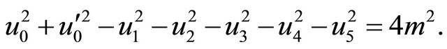 (29)
(29)
This expression has the form of a “mass hyperboloid” with an  symmetry. However, we have to keep in mind that on the hyperboloid (29) there are no symmetry operations that “rotate” a spatial component of P into a spatial component of
 . So the values of
  and
and  are separately kept constant under all (permitted) symmetry operations.
Nevertheless, we can obtain rotations of spatial components of P into such of q, provided that the timelike components P0 and q0 are automatically adjusted. Then the values of  and
and  are again separately kept constant. We will take advantage of this possibility below.
Considered as a hyperboloid with full  symmetry, the domain (29) is isomorphic to the quotient group
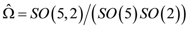 , which is a homogeneous domain with a transitive action of
 . With the group actions of the full
 , (29) is an unbounded realization of the abstract manifold
 . If we restrict the group action to
  and
and , then (29) is an unbounded realization of our parameter manifold
 .
.
A well-known bounded realization of the homogeneous domain  is the complex Lie ball [11,16]
 (30)
(30)
The boundary of  is given by
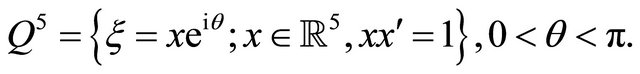 (31)
(31)
(The vector  is the transpose of
 ,
, ![]() is the complex conjugate of
is the complex conjugate of .) The Lie ball is included in the complex unit ball
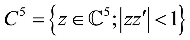 (32)
(32)
and contains the real unit ball
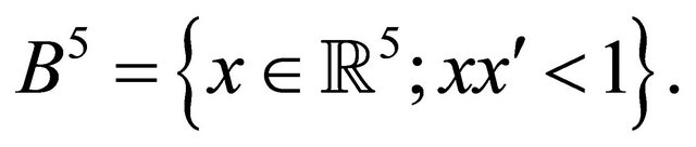 (33)
(33)
The complex unit ball is isomorphic to the upper halfspace of , whereas the Lie ball is isomorphic to the forward light cone in 5 + 2 dimensions.
There is some similarity to the mapping of the (unbounded) complex plane into the (bounded) Riemann sphere by a Möbius transformation. Möbius transformations are conformal transformations. They leave invariant the form of volume elements but they change their sizes. Whereas a subdomain of the complex plane may have an infinite volume, the volume of its image in the Riemann sphere is finite. The Riemann sphere without the image of “infinity” has the same non-compact topology as the complex plane, but is bounded. By adding the image of infinity, the Riemann sphere becomes compact (this is the compactification of the complex plane). On the internet, a very instructive animation of the Möbius transformation can be found [17]. Readers not familiar with Möbius transformations or the Riemann sphere may want to load the video of this animation before continuing.
Since the unbounded as well as the bounded realizations are true realizations of , they are isomorphic. Both can be used to parametrize a (fictive)
  invariant state space, but the bounded realization
  of
of  has the advantage that it provides a finite environment for calculating the Lebesgue integral (19). Therefore, the following evaluation of this integral will be based on the bounded realization of
 .
.
We can separate the integral into a spherical integral over the surface  and a second integral over the radial direction of
 . The spherical part is given by
 (34)
(34)
The normalization of this integral requires the factor
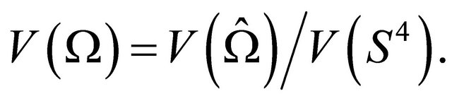
 , where
  is the volume of
 . This delivers a first contribution of
  to
to .
.
We can immediately integrate over the phase  on the boundary (31), which to
  adds a factor
![]() , and allows replacing the volume element
, and allows replacing the volume element  by
by  with real parameters x.
Next we have to add the integration in the radial direction of . As indicated above, we want to obtain the infinitesimal volume element as a Cartesian volume element. Mapping a spherical volume to a rectangular one includes a step that is known as the “quadrature of the circle”. (As an example: the volume of the unit ball in three dimensions equals the volume of a cube with edge length
 .)
.)
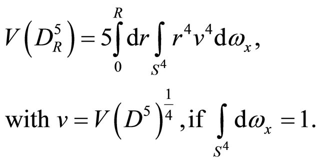
Consider the formula that relates the volume of a Lie ball  with radius R to the volume of the unit Lie ball
 (35)
(35)
When we project the volume of  onto the real ball
  with surface
 , then
  can be expressed by the integral
 (36)
(36)
A rectangular volume with the same numerical value is given by
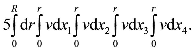 (37)
(37)
This integral is an analogue to the “quadrature of the circle”. Unfortunately, it maps the volume of the Lie ball not to a cube, but to the cuboid
 (38)
(38)
The infinitesimal volume element  of integral (36) (e.g. at
 ) is accordingly mapped to the infinitesimal volume element of integral (37)
 (39)
(39)
Consequently, to obtain an isotropic volume element, the coordinate in the radial direction must be replaced (rescaled) according to
 (40)
(40)
Therefore, to extend the 4-dimensional volume element  to a five-dimensional Cartesian isotropic volume element
 , we have to multiply
  by the right hand side of relation (40). This adds a factor of
 to
to .
.
The fifth dimension also adds a factor to the normalization of the projection operator, but for the Lie ball of radius 1 this factor is equal to 1, as can be seen by inspection of integral (37).
The infinitesimal volume element now refers to the full  -symmetric manifold
 , but remember that the original manifold
  is subspace of
  that is generated by rotations around four rotational axes instead of five. Therefore, the volume of
  is smaller by a factor equal to the volume of the quotient group
  , which is isomorphic to the real unit sphere
  in five dimensions (cf. e.g. [18]). Hence,
 (41)
(41)
However, there is no indication that the perturbation algorithm excludes the integration over the direction of . Therefore, we cannot do other than keep this integration, together with the corresponding normalization volume
 . Keeping the five dimensions of the volume element means that on
  we integrate through the P-q boundary (on an integration path that connects
  with
with ). Thereby we add up more points of the parameter space than the one-to-one relation between the parameter space and the state space allows. But, as indicated above, these additional point are valid parameter combinations provided that the timelike components are determined “automatically”. This is indeed the fact, because the integration variables are the space-like components, whereas the timelike components are determined from them via the mass shell relations. If we perform the same five-dimensional integration in the
 ![]() matrix element (12), we add up multiple copies of states, with multiplicity given by the volume of
matrix element (12), we add up multiple copies of states, with multiplicity given by the volume of . We can compensate for the extra copies by simply adjusting the normalization of each state by a common factor and include this factor beforehand in the infinitesimal volume element. This adds a factor of
  to
to .
.
This is a trick that works well with a projection operator that integrates with equal weights over the full parameter space. But it conceals the fact that we are evaluating a five-dimensional integral over a basically four-dimensional manifold. This discloses an inherent weakness in the perturbation algorithm of QED, which becomes obvious when the first order term is iterated: The evaluation of higher order terms involves contractions (permutations) of creation and annihilation operators. Thereby the structure of the projection operator gets lost and may become replaced by one of the notorious divergent loop structures of QED. Then the extra integration through the P-q boundary cannot be compensated for as easily as before. It becomes visible as an extra degree of freedom, leading to ill-defined integrals, which call for another trick to “regularize” them. (A regularization method, based on distribution theory, can be found in Scharf [10].) The insight into the mechanism that may lead to these divergences points out a way to solve the divergence problem right at its source—but that means reengineering the perturbation algorithm, which is not the subject of this paper.
So far we have ignored spin degrees of freedom. When we include spin, the number of possible intermediate two-particle states is extended by a factor of 4, due to the 2 × 2 spin states of the electrons. In a scattering experiment, additional states open up additional channels for transitions. Therefore, the empirical value of the coupling constant ![]() should be four times larger than the value of
should be four times larger than the value of , calculated without spin degrees of freedom, indicates. To allow for a comparison with the empirical value, we therefore add a factor of 4 to
 . This is a somewhat heuristic argumentation. A more in depth discussion would probably require a precise analysis of experimental setups, which at present is beyond the author’s capabilities.
When we replace the total and relative momentum by the individual particle momenta  and
and , the Jacobian
 (42)
(42)
contributes a factor of 2 to the infinitesimal volume element.
Collecting all factors results in a total weight factor  of
of
 (43)
(43)
Expression (43) is identical to Wyler’s semi-empirical formula, which here has been derived by reverse engineering the perturbation algorithm of QED.
Finally, we map the normalized volume element, constructed on the bounded realization, into the unbounded realization by a stereographic projection ,
,
 (44)
(44)
The transformation (44) is a conformal mapping. The proof is by writing down (44) for an infinitesimal cube. Therefore, the isotropic volume element  is mapped onto the isotropic Cartesian volume element
  in
in . The value of
  is not touched by this mapping. (A more intuitive, though less elegant, way would be to replace the unit Lie ball by a Lie ball with radius
  and then let
 .)
.)
The volumes  and
and  in Wyler’s formula (43) have been calculated by Hua [16]. With
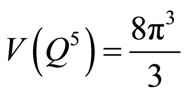 (45)
(45)
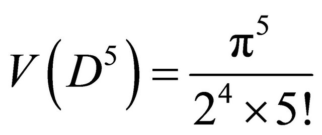 (46)
(46)
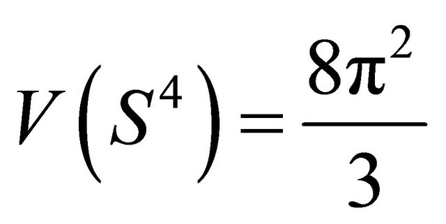 (47)
(47)
we obtain
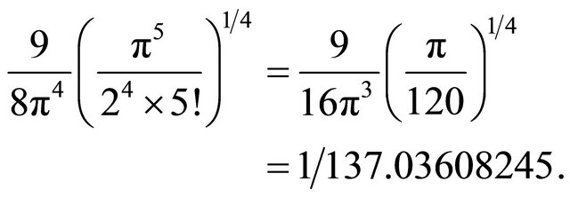 (48)
(48)
This value agrees up to a factor of 0.9999995 with the experimental (low energy) value of![]() , which is the reciprocal of 137.035999084 (51) [19].
, which is the reciprocal of 137.035999084 (51) [19].
Note that, while deriving Wyler’s formula, we have not touched the integrand of integral (12), which contains the “physics” of the S matrix. The whole calculation was based on the geometrical properties of the parameter space only, without any direct involvement of the state space. The operations on the parameter space, especially the mapping onto a finite domain and back onto the infinite momentum space, followed transparent mathematical rules. Therefore, we can be sure that we did not inadvertently modify the physical contents of the S matrix.
The extremely close agreement of  with the (low energy) empirical value of
 ![]() is a strong experimental indication that the (low-energy) “physical” two-particle state space of elastic e-e scattering in fact matches an irreducible two-particle representation (of identical, massive, spin-
is a strong experimental indication that the (low-energy) “physical” two-particle state space of elastic e-e scattering in fact matches an irreducible two-particle representation (of identical, massive, spin- particles) of the Poincaré group. Since Joos’s paper [20] on the representations of the Lorentz group, these representations have been generally known.
Moreover, the numerical value of ![]() can be regarded as a kind of checksum that double-checks the decisive steps of the reverse engineering procedure presented above. In fact, the individual elements of Wyler’s formula helped the author more than once to avoid dead ends.
can be regarded as a kind of checksum that double-checks the decisive steps of the reverse engineering procedure presented above. In fact, the individual elements of Wyler’s formula helped the author more than once to avoid dead ends.
The volume element on  still has only five dimensions, compared to six for the volume element
  in the expression (12) of the
 ![]() matrix. This shortfall can easily be resolved, without affecting the
matrix. This shortfall can easily be resolved, without affecting the ![]() matrix, by simply extending the volume element of
matrix, by simply extending the volume element of  to a sixdimensional one. This is because, in a two-particle scattering process, we can always orient the reference frame in such a way that the sixth momentum component of the incoming state is identically zero. So a six-dimensional volume element in (12) has only the “cosmetic” advantage of making the
 ![]() matrix look explicitly covariant.
matrix look explicitly covariant.
Wyler’s formula defines a geometrical factor that relates an irreducible two-particle representation of the Poincaré group to a two-particle product representation, just as ![]() relates the circumference of a circle to its diameter. In relating this geometrical factor to the empirical fine-structure constant, we have to keep in mind that the latter is determined experimentally. Therefore, all orders of the perturbation series, including non-elastic processes, contribute to its value. The accumulation of these contributions is described by the renormalization group. This leads to a weakly energy dependent “effective” coupling constant—the “running coupling constant”. At low energies, and depending on the experimental setup, nonelastic contributions of “infrared photons” can be kept well under control. Therefore, the fine-structure constant measured by low-energy e-e scattering comes close to the calculated value of the coupling constant for elastic scattering. This explains the success of Wyler’s formula in reproducing the empirical value of
relates the circumference of a circle to its diameter. In relating this geometrical factor to the empirical fine-structure constant, we have to keep in mind that the latter is determined experimentally. Therefore, all orders of the perturbation series, including non-elastic processes, contribute to its value. The accumulation of these contributions is described by the renormalization group. This leads to a weakly energy dependent “effective” coupling constant—the “running coupling constant”. At low energies, and depending on the experimental setup, nonelastic contributions of “infrared photons” can be kept well under control. Therefore, the fine-structure constant measured by low-energy e-e scattering comes close to the calculated value of the coupling constant for elastic scattering. This explains the success of Wyler’s formula in reproducing the empirical value of![]() .
.
7. Angular Momentum and Entanglement
Although we have identified the two-particle state space as an irreducible representation of the Poincaré group, it is not yet clear why the intermediate states in the S matrix are entangled. What explains the obvious absence of simple (separable) product states in the intermediate states?
Remember that we have based the calculation of  on the observation that there is an internal rotational degree of freedom. This corresponds to an internal angular momentum of a two-particle state.
Irreducible representations of the Poincaré group are characterized by eigenvalues of the invariant (Casimir) operators (see e.g. Schweber [21])
 (49)
(49)
and
 (50)
(50)
Here  and
and  are the operators of fourmomentum and four-dimensional angular momentum, respectively.
To define a basis of the state space of an irreducible representation, we have to select a complete commuting set of operators. Such a set consists of the momentum operators  and one of the components of
 , say
, say , the component of the angular momentum operator in the direction of
 . The states of this basis can then be labeled by the quantum numbers of
  and
and .
.  is the generator of rotations with
  as the rotational axis. To give a two-particle state the property of an eigenstate of
 , it is required that this state be a linear combination of all (pure) product states that can be reached from a given product state by such a rotation. This necessarily gives a two-particle base state an entangled structure. (Therefore, the separable states (13), although used to generate irreducible two-particle states, do not form a basis of an irreducible two-particle state space.)
Entanglement correlates the individual particle states within the two-particle state. Obviously, it is this correlation that is observed as electromagnetic interaction.
8. Vector Potential
In Feynman’s formulation of the perturbation algorithm, the electromagnetic field operators have a surprisingly marginal role. In fact, Feynman deliberately eliminated these operators from the algorithm, to formulate it “as a description of a direct interaction at a distance (albeit delayed in time) between charges” [7]. This underlines the auxiliary role of the vector potential within QED.
In setting up the perturbation algorithm, the Dirac equation of the free electron is modified by adding a “quantized vector potential” to the momentum, in the sense of a “minimal coupling to the electromagnetic field”. Within the perturbation algorithm, the vector potential then obviously has the sole task of generating entangled states from incoming states. After having accomplished this, it is eliminated.
Based on this simple functionality, the reverse engineering approach must understand the quantized vector potential as a sophisticated mathematical tool with the following properties:
a) It modifies the Dirac equation by a “bookkeeping” operator that stands for the “potential” that the state  may be changed, to become again a solution of the Dirac equation, but with the momentum
 .
.
b) This change becomes active when and only when the operator  encounters its counterpart
 .
.
The intended(!) result is that within the perturbation algorithm, two (incoming) single-particle states are mapped onto an entangled two-particle state with the same total momentum as the incoming states. In this way a quantum mechanical transition from an incoming separable product state to a state of the corresponding irreducible two-particle representation is described.
The fact that  enters as a “perturbation” to the momentum
 ![]() in the Dirac equation, rather than, e.g., to the
in the Dirac equation, rather than, e.g., to the  -term, explains why the S matrix contains
  - matrices, something which, in a projection operator, is somewhat unexpected. The strict pursuit of this perturbation ansatz, necessarily places the
  -matrices in the S matrix. The details can be found in any good textbook on QED (see e.g. Schweber [22]).
9. Virtual Particles, Vacuum Fluctuations, and All That
Feynman coined the term “virtual quantum” in his 1949/ 1950 papers. Later it was replaced by “virtual particle”. It corresponds to the c-number that is left when the creation and annihilation operators of the same particle type are permuted. In Feynman graphs, these c-numbers are represented by internal lines connecting two vertices. In the momentum representation, these c-numbers are essentially ![]() functions that ensure momentum conservation between two vertices.
functions that ensure momentum conservation between two vertices.
In evaluating S matrix elements, Feynman used the commutation relations to shift the creation and annihilation operators through the expression of the matrix element, until they hit the vacuum state and thereby annihilate themselves. In higher orders of the perturbation series, this leads to more and more “virtual particles”.
The notion of “virtual particle” has triggered speculations about the “physical” nature of virtual particles. It has been tried to give virtual particles some reality by considering them as particles that have “left their mass shell”. It has even been argued that, because of Heisenberg’s uncertainty principle, virtual particles may become “real” for short periods of time. (Ignoring the fact that this principle refers to particles, not to ![]() functions.) Together with the conviction that QED is the prototype of a quantum field theory, such ideas, although unsubstantiated, have strongly influenced the way we still think about QED and particle physics in general. Thereby they have unfortunately clouded our view of the comparatively simple mathematics of the perturbation algorithm for more than six decades.
functions.) Together with the conviction that QED is the prototype of a quantum field theory, such ideas, although unsubstantiated, have strongly influenced the way we still think about QED and particle physics in general. Thereby they have unfortunately clouded our view of the comparatively simple mathematics of the perturbation algorithm for more than six decades.
The foregoing analysis is fully in line with Feynman’s original notion of a virtual quantum, and it is evident that in a simple and transparent product state space there is no room for speculations about ![]() functions becoming particles, or “physical particles” being “dressed” by clouds of particle/antiparticle pairs “created from the vacuum”.
functions becoming particles, or “physical particles” being “dressed” by clouds of particle/antiparticle pairs “created from the vacuum”.
The “vacuum state” used in the Fock space formalism is a symbolic state that only in connection with creation operators acting on it has a counterpart in physical reality. By reverse engineering, we have found that the “physical” state space is nothing other than a two-particle subspace of the Fock space. Therefore, in QED there is no “physical” vacuum other then the (symbolic) vacuum of the Fock space.
A last remark concerns “vacuum fluctuations”. There are “vacuum graphs”, which have internal lines, but no external (incoming or outgoing) lines. Attempts have been made to understand these graphs as manifestations of quantum mechanically caused “vacuum fluctuations”. The mathematical contents of these graphs (in the momentum representation) are essentially a product of ![]() functions, whose arguments are momenta. Therefore, they provide us, if at all, with the insight that, even when no particles are present, the principle of momentum conservation is observed.
functions, whose arguments are momenta. Therefore, they provide us, if at all, with the insight that, even when no particles are present, the principle of momentum conservation is observed.
Regarding the wide-spread opinion that the Casimir effect “proves” the existence of vacuum fluctuations, the reader is referred to Jaffe’s article [23].
10. Higher Orders
Our analysis of QED has so far been based on the first order of the perturbation series. Higher orders are obtained by iterating the first order operator. Therefore, they are mathematically completely determined by the properties of the lowest order.
The iteration process is inherent to every perturbation approach. What is special about a system of fermions, is that the anticommutation relations allow interchanging the creation and annihilation operators. Feynman has taken advantage of this property to set up practicable rules for evaluating S matrix elements. In higher orders, these rules lead to a large variety of topologically different Feynman graphs. Some of them have been interpreted as “virtual pair creation” or “vacuum polarization”. It is evident from our analysis of the two-particle S matrix that intermediate states are nothing other than two-particle states, which do not give space for any additional pairs of particles “created from the vacuum”. So these interpretations merely give certain topological properties of Feynman graphs catchy names.
11. Discussion
The reverse engineering approach has led us to more than just a description of the perturbation algorithm. The new insights into its mathematics, gained in this way, allows calculating the electromagnetic coupling constant![]() . The close agreement of the calculated with the empirical value provides evidence that the disclosed mathematical structure indeed reflects physical reality—more than current concepts of interacting fields do, which leave the values of coupling constants undetermined. It reveals that in the perturbation algorithm of quantum electrodynamics, the S matrix has the function of a projection operator onto intermediate irreducible two-particle states, with
. The close agreement of the calculated with the empirical value provides evidence that the disclosed mathematical structure indeed reflects physical reality—more than current concepts of interacting fields do, which leave the values of coupling constants undetermined. It reveals that in the perturbation algorithm of quantum electrodynamics, the S matrix has the function of a projection operator onto intermediate irreducible two-particle states, with ![]() acting as a normalization factor for these states.
acting as a normalization factor for these states.
With this understanding of the mathematical structure of the S matrix, we can say: The S matrix describes a transition from a separable product state of two incoming electrons (preparation) to an intermediate irreducible two-particle state (propagation) and then back to a separable product state of two outgoing electrons (analysis).
The formation of irreducible intermediate states can be understood as the manifestation of a general rule of relativistic quantum mechanics: An isolated quantum mechanical system is described by an irreducible representation of the Poincaré group. Therefore, the physical effects described by the S matrix can be fully explained by elementary principles of relativistic quantum mechanics.
Whereas in the traditional interpretation of QED, the entanglement of two-particle states is caused by an exchange of “virtual gauge particles”, it has been shown that entanglement is a natural property of the state space of an irreducible two-particle representation of the Poincaré group. Since we have not touched the mathematical structure of QED, we have thereby traced back the gauge invariance structure of QED to basic rules of quantum mechanics and Poincaré invariance. However, now gauge invariance goes together with a certain value of the coupling constant, and we are lucky enough that this value matches the (low energy) value of the empirical finestructure constant.
Wyler’s work has been of crucial importance for the foregoing analysis, because it has guided the author to valuable mathematical tools that used to be outside the horizon of a theoretical physicist. Therefore, some of the objections that in the past were raised against Wyler’s mathematics should be commented on. A major objection was that Wyler used certain bounded spaces with a radius equal to 1. It was argued (Robertson [13]), that “there is no known reason for setting ”, and it was suspected that a different radius would yield a different value for
![]() . Another point of criticism was that Wyler could not clearly specify how the fourth-root factor entered his calculation.
. Another point of criticism was that Wyler could not clearly specify how the fourth-root factor entered his calculation.
From the derivation of Wyler’s formula presented here, it should be clear that it does not depend on the radius of the Lie sphere. The reason is that by Equation (18) the weight factor  is defined as the quotient of two infinitesimal volume elements on the surface of the twoparticle mass hyperboloid. Whether we map these volume elements to a Lie sphere with radius 1 or any other radius or do not map it at all, does not have any influence on this quotient. Speaking generally, the volumes in Wyler’s formula are not the outcome of the mapping onto the Lie sphere, but rather reflect the internal geometrical structure of the homogeneous domain
  , which is independent of any mapping. The fourth-root factor has been identified as a trivial conversion factor relating a spherical to a Cartesian volume element.
In an answer to Robertson’s objections, Gilmore wrote [24]:
“Wyler’s work has pointed out that it is possible to map an unbounded physical domain—the interior of the forward light cone—onto the interior of a bounded domain on which there also exists a complex structure. This mapping should prove of immense calculational value in the future.”
12. Conclusions
The empirical value of ![]() provides experimental evidence that the state space of two interacting electrons belongs to an irreducible two-particle representation of the Poincaré group.
provides experimental evidence that the state space of two interacting electrons belongs to an irreducible two-particle representation of the Poincaré group.
The electromagnetic interaction can, therefore, be fully understood within the framework of a “free” relativistic multi-particle quantum theory, without the need to postulate an interaction with a “gauge field”—provided that a general rule of relativistic quantum mechanics is observed: Isolated systems are described by irreducible representations of the Poincaré group.
13. Acknowledgements
I would like to thank several unknown referees for their critics, which helped me to improve my presentation. Special thanks go to Freeman Dyson for having read a previous version of the manuscript, and to Armand Wyler for his encouraging comments. Last not least, I am grateful to Werner Heisenberg, who more than forty years ago granted me a postgraduate studentship of the Max Planck Society. During my stay at the Max Planck Institute for Physics and Astrophysics, the first ideas of this work came about [25].
REFERENCES
- W. Smilga, Journal of Physics: Conference Series, Vol. 343, 2012, Article ID: 012112. doi:10.1088/1742-6596/343/1/012112
- R. Haag, Matematisk-Fysiske Meddelelser Udgivet af. Det Kongelige Danske Videnskabernes, Vol. 29, 1955, pp. 1-37.
- N. D. Mermim, Physics Today, Vol. 57, 2004, pp. 10-12. doi:10.1063/1.1768652
- E. Eilam, “Reversing: Secrets of Reverse Engineering,” John Wiley & Sons, Hoboken, 2005.
- Wikipedia, “Reverse Engineering.” http://en.wikipedia.org/wiki/Reverse_engineering
- R. P. Feynman, Physical Review, Vol. 76, 1949, pp. 749- 759. doi:10.1103/PhysRev.76.749
- R. P. Feynman, Physical Review, Vol. 76, 1949, pp. 769- 789. doi:10.1103/PhysRev.76.769
- R. P. Feynman, Physical Review, Vol. 80, 1950, pp. 440- 457. doi:10.1103/PhysRev.80.440
- W. Heisenberg, Zeitschrift für Physik, Vol. 120, 1943, pp. 513-538.
- G. Scharf, “Finite Quantum Electrodynamics,” Springer, Berlin, Heidelberg, New York, 1989. doi:10.1007/978-3-662-01187-4
- A. Wyler, Comptes rendus de l’Académie des Sciences, Vol. 271A, 1971, pp. 186-188.
- R. Gilmore, “From a Visit to Armand Wyler in Zürich.” http://www.tony5m17h.net/WylerHua.html
- B. Robertson, Physical Review Letters, Vol. 27, 1971, pp. 1545-1547. doi:10.1103/PhysRevLett.27.1545
- D. J. Gross, Physics Today, Vol. 42, 1989, pp. 9-11. doi:10.1063/1.2811237
- E. B. Vinberg, “Homogeneous Bounded Domain,” Encyclopedia of Mathematics, Springer. http://www.encyclopediaofmath.org/index.php?title=Homogeneous_bounded_domain
- L. K. Hua, “Harmonic Analysis of Functions of Several Complex Variables in the Classical Domains,” Translations of Mathematical Monographs, Vol. 6, American Mathematical Society, Providence, 1963.
- Link to animation of Möbius transformation: http://www.ima.umn.edu/videos/mobius.php
- I. S. Sharadze, “Sphere,” Encyclopedia of Mathematics, Springer. http://www.encyclopediaofmath.org/index.php?title=Sphere
- D. Hanneke, S. Fogwell and G. Gabrielse, Physical Review Letters, Vol. 100, 2008, Article ID: 120801. doi:10.1103/PhysRevLett.100.120801
- H. Joos, Fortschritte der Physik, Vol. 10, 1962, pp. 65- 146. doi:10.1002/prop.2180100302
- S. S. Schweber, “An Introduction to Relativistic Quantum Field Theory,” Harper & Row, New York, 1962, pp. 36- 53.
- S. S. Schweber, “An Introduction to Relativistic Quantum Field Theory,” Harper & Row, New York, 1962, pp. 272- 280.
- R. L. Jaffe, Physical Review, Vol. D72, 2005, Article ID: 021301.
- R. Gilmore, Physical Review Letters, Vol. 28, 1972, pp. 462-464. doi:10.1103/PhysRevLett.28.462
- W. Smilga, “Lokale Eigenschaften von Vielteilchensystemen in einer de Sitter-Invarianten Quantenmechanik,” Dissertation, Eberhard-Karl-Universität, Tübingen, 1972.
NOTES
*Parts of this article were presented at the 7th International Conference on Quantum Theory and Symmetries (QTS7) in Prague 2011 [1].