ABSTRACT

A new approach to classical statistical mechanics is presented; this is based on a new method of specifying the possible “states” of the systems of a statistical assembly and on the relative frequency interpretation of probability. This approach is free from the concept of ensemble, the ergodic hypothesis, and the assumption of equal a priori probabilities.

1. Introduction

The object of classical statistical mechanics is to explain the (statistical) properties of an assembly of a large number of identical particles in terms of the (deterministic) laws of classical mechanics. Such a theory has been developed by Gibbs in the first decade of the last century [1]. The Gibbs approach, presented by Tolman [2], has been accepted as the conventional approach to classical statistical mechanics. The theory presented by Tolman and the subsequent authors [3,4] is based on: 1) the concept of “state” of a many-particle system as defined by classical mechanics in the sense that the state of a N-particle system at any instant of time can be specified by a point in 6N dimensional phase space and 2) the notion of probability prevalent at the beginning of the last century according to which probability refers to a manyparticle system “chosen at random from the ensemble” of many-particle systems.

In this paper we present a new approach to classical statistical mechanics based on the significant progress made during and after the third decade of the last century in the theory of probability (a branch of pure mathematics) and the methods of statistical analysis (a branch of applied mathematics) [5,6]. This new approach is based on: 1) a new method of specifying the possible “states” of an assembly of particles which (method) is consistent with the requirements of statistical analysis, and 2) on the relative frequency interpretation of probability. The present approach is an independent approach and should be viewed as such. For the sake of clarity, the distinctive features of the two approaches are also discussed in the text.

2. Preliminary Considerations

For the sake of clarity we may just mention the main features of statistical analysis and the relation between statistical analysis and probability theory. A large number of physical entities (such as adult men in a population) are said to form a collective, or a population, or a statistical assembly [5], if each entity (or member) of the assembly exists in one of the many (at least two) possible states S_n’s (such as the state of parenthood of having n number of children) and the states of the members collected in any systematic manner lead to a random sequence of these possible states, in which each entry belongs to one member. If N_n is the number of times the state S_n occurs in the random sequence having a total number of N₀ entries, then N_n/N₀ is the relative frequency of the state S_n. As there can be many different systematic ways of collecting the data, there would be many random sequences of the same states (relevant to the given assembly). In all these random sequences the relative frequencies of the states would have approximately (in the statistical sense) the same set of values; such sequences are said to be statistically equivalent. One important feature of all statistical properties is that they are independent of such details as: 1) which particular member of the assembly is in which particular state, 2) the regions of space within which the individual members exist in the assembly (such as the places of residence of men), and 3) the total number of members of the assembly. Evidently, the relative frequencies of the possible states in a random sequence possess these properties.

In the theory of probability, statistical properties are dealt with in a more abstract and general manner by associating probabilities with the possible states per se; these probabilities are treated as unspecified constants with the understanding that, with reference to any random sequence of states (relevant to a statistical assembly), the numerical values of the relative frequencies of the states in the sequence are approximately equal to the numerical values of the corresponding probabilities. It is extremely important to appreciate the point that (the relative frequencies as well as) the probabilities are associated with the possible states and not with the members of the assembly. With this background we consider classical statistical mechanics.

A physical entity having finite non-zero mass bound to a time-independent potential is said to form a conservative system; to the extent the internal structure and the external dimensions of the entity do not play any role in the phenomenon under consideration, we can regard the entity as a particle, a point-mass. We can attribute many physical properties to such a system; the sum-total of all the physical quantities which can be attributed to the system at any instant of time is said to specify fully the “instantaneous state” of the system at that instant. As time passes, the system evolves through a continuous sequence of successive instantaneous states as governed by the laws of classical mechanics; such a sequence may be called a dynamical state of the system. Each dynamical state is determined by one solution of Newton’s second law of motion which (solution) is specified by two constants, r₀ and p₀ , the position and the momentum of the particle at some “initial” instant of time t₀. A dynamical state may be denoted as S(r₀, p₀, t₀; r, t) which gives the position r of the particle as a function of time t ; once r is given as a function of time, all the physical quantities attributable to the system at any instant t, as well as their variations with t, can be derived mathematically from the function. In the case of a conservative system in a dynamical state, the energy E of the system remains constant so long as the system is in that dynamical state. There can be infinite number of such possible dynamical states for the given system, though a system exists, over a duration of time, in only one possible dynamical state. In some special cases, the system (such as a simple or conical pendulum, or a particle in a closed Kepler orbit) may go repeatedly through the same sequence of successive instantaneous states; such a dynamical state may be called a cyclic dynamical state.

Our object of study in classical statistical mechanics is a statistical assembly consisting of a large number of identical independent conservative systems which obey the laws of classical mechanics. Such systems may be: free particles (helium atoms), rigid rotators (diatomic molecules), harmonic oscillators (atoms in a crystal lattice), etc. In all these cases, first we have to identify the possible states of the systems relevant to the statistical properties of the given assembly and then use the laws of probability to determine the probabilities associated with these states. As our object is to present the new approach, we consider only an assembly of free particles.

3. An Assembly of Free Particles in Statistical Equilibrium

For the sake of definiteness let us consider an assembly of a large number N₀ of identical particles confined (by what is normally referred to as the walls of a container) within a fixed volume of field-free space of macroscopic dimensions. Evidently, over a duration of time each particle would be in a dynamical state characterized by a pair of constants such as r₀, p₀, with the understanding that all such pairs of constants specifying all the possible dynamical states (of all the particles) correspond to the same initial instant of time t₀. Though we have referred to them as particles, they are indeed physical entities having non-zero spatial extension and hence they would collide with one another exchanging energy and momentum. As a result, a particle would travel along a segment of a straight line belonging to a particular dynamical state, collide with another particle, exchange energy and momentum, make a transition to another particular dynamical state, travel along a segment of a straight line belonging to the new dynamical state to collide again, and so on; every particle would go through such a process incessantly. It is envisaged that as a result of such repeated transitions (from one dynamical state to another) made by all the particles over a sufficiently long initial duration of time, a “state of dynamic equilibrium” would be reached in the sense that the fractions of the total number of particles of the assembly in different possible dynamical states would remain almost constant over subsequent durations of time. Such an assembly is said to be in statistical equilibrium. Our interest is only in the equilibrium state and not in how equilibrium is reached from an initial non-equilibrium state [7].

As mentioned at the outset, first we have to specify the possible states of the particles in a manner that is consistent with the laws of classical mechanics as well as with the methods of statistical analysis. According to classical mechanics, the dynamical state of a (free) particle between two successive collisions is specified by the momentum of the particle and by the coordinates of the particle at the two points of collision. According to the methods of statistical analysis the positions of the particles within the volume of space of the assembly have no relevance to the statistical properties of the assembly. This means that, so far as the statistical properties of the assembly are concerned, we need specify each possible state by momentum only. We refer to them as momentum states. Evidently, the possible values of momentum p have a continuous range (both in magnitude and direction).

We associate probability P(p) dp with the states corresponding to momentum lying between p and p + dp; here dp is an element of constant magnitude dp_x dp_y dp_z. Evidently, P(p) corresponds to unit interval of p values. Our object now is to find this probability distribution using the laws of probability and the methods of statistical analysis. We treat (to begin with) P(p) as an unspecified function of p and then derive a general expression for it by making use of the properties of the equilibrium state of the assembly and the results of probability theory.

If we consider at any one instant of time t₁, the states of different particles (which exist at different points within the volume of the assembly) one after the other in any systematic manner, we get a random sequence of the possible momentum states p’s. This random sequence has N₀ number of elements corresponding to N₀ number of particles in the assembly. If the states corresponding to momentum lying  between p and p + dp occur N₁(p) number of times in the sequence, the relative frequency w₁(p) = N₁(p)/N₀ of these states in the sequence  would be approximately (in the statistical sense) equal to the probability P(p) dp. If we consider the states at another instant of time t₂ (after an interval of time long enough for particles to undergo transitions) we get another random sequence of the same states in which also the relative frequency w₂(p) is approximately equal to the probability P(p) dp. Such random sequences are statistically equivalent. Thus because of the dynamic nature of equilibrium, we get a large number of statistically equivalent random sequences of the same states p’s, the random sequences being relevant to the “state” of the assembly at the instants of time t₁, t₂,.

Let us consider the random sequence at the instant of time t₁. Now we define (what is referred to in statistical analysis [5,6] as) a binomial random variable R(p) which assumes the value 1 if a state in the random sequence belongs to momentum between p and p + dp and assumes the value 0 if it does not. This leads to a (derived) random sequence of 1’s and 0’s. Evidently, R(p)  is the total number N₁(p) of the particles having momentum between p and p + dp at the instant t₁. Corresponding to the random sequence at t₂, we get another value N₂(p). 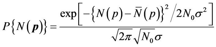Thus corresponding to random sequences at different instants of time t₁, t₂, , we get different values of N(p). Since a well defined (time-independent) probability P(p) dp is associated with the states between p and p + dp, these values of N(p) would have a well defined distribution characterized by the probability P(p) dp. According to the central limit theorem of the probability theory [5,6], the probability P{N(p)} that the quantity SR(p)  has (at the conceptual instant of time) the value N(p) is given by

, (1)

where (p) is exactly equal to P(p) dp N₀ and (p) = P(p) dp {1 – P(p) dp}. Here (p) is the most probable value and, the distribution being symmetric, (p) is also the mean value of N(p) taken over this distribution (which, in effect, is over a duration of time); σ is the standard deviation. This shows that because of the dynamic nature of the equilibrium distribution, the number N(p) of particles having momentum between p and p + dp fluctuates leading to a time-independent Gaussian distribution of values with the mean value (p) and the standard deviation σ. Evidently, this is true of each possible value of p.

It is interesting to consider the state of a particular single particle of the assembly at different instants of time. Because of collisions, the particle would be in different momentum states at different (well separated) instants of time, leading to a random sequence of momentum states; this sequence would have the same number of elements as the number of instants of time at which the state of the particle is considered. Since the probability distribution P(p) dp is associated with the possible states per se (and not with the particles) this random sequence would be statistically equivalent to the random sequence of states of the particles of the assembly at one instant of time. So, the relative frequency distribution w(p) in any long segment of this sequence also would be approximately equal to the probability distribution P(p) dp. We may regard this sequence as being made up of a large number of successive segments each segment having n₀ number of elements. With reference to the first segment, R(p) is the total number n(p)₁ of instants of time (out of n₀ number of instants) at which this particle has momentum between p and p + dp; with reference to the second segment we get another number n(p)₂; and so on. All these numbers are approximately equal to P(p) dp n₀. These numbers lead to a Gaussian distribution similar to (1). Again, the mean number of instants of time (p) (out of a total number of instants of time n₀) at which the particular particle has momentum between p and p + dp is exactly equal to P(p) dp n₀. This is true of every possible momentum p of this particular particle under consideration. All this is true also of every other particle in the assembly. Significance of this result is that the mean value of a physical quantity taken over the states of a large number of particles of the assembly at any one instant of time is approximately equal to that taken over the states of any one particular particle at equally large number of instants of time.

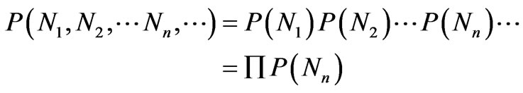
A particle makes a transition to another momentum state, p' say, as a result of its collision with another particle and this process is independent of the momentum states of all the other particles in the assembly. So the fluctuations in the number N(p') of particles having momentum between p' and p' + dp would be independent of the fluctuations in the numbers relevant to all other momentum values (except for the weak condition that the sum of these numbers should remain constant at N₀). So, the probability P{N(p')}, given by (1), that N(p') number of particles have momentum between p' and p' + dp is independent of the probability P{N(p'')} that N(p'') number of particles have momentum between p'' and p'' + dp for any two distinct values of momentum p' and p''. The probability P{N(p)}for one value of p being independent of that for another value, the probability P(N₁, N₂, , N_n,) that N₁ number of particles have momentum between p₁ and p₁ + dp, and N₂ between p₂ and p₂ + dp, , N_n between p_n and p_n + dp, , is given by

(2)

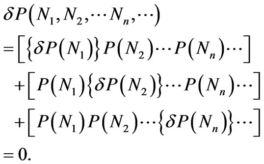
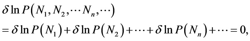
This is a multi-dimensional Gaussian distribution and its maximum (which corresponds to each N_n being equal to, the most probable value) may be specified by the condition

(3)

Here each term has not only the condition for the probability relevant to one value of momentum p being maximum, but also the probabilities relevant to all the other values as well. Thus the condition (3) is not consistent with the fact that the probabilities P(N_n)’s are all independent of one another. So we consider, instead, the condition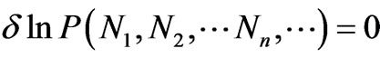. We have

(4)

where each term refers to one value of momentum only, consistent with P(N_n)’s being independent of one another. Thus though both the conditions (3) and (4) look mathematically equivalent, only the condition (4) is physically appropriate. Importance of this result cannot be overemphasized.

All that has been said so far is mere explication, in terms of the laws of probability, of what we should mean by (dynamic) statistical equilibrium, once we assume that time-independent probabilities associated with the possible “states” of the particles exist; in fact, no law physics is involved. A little reflection would show that the above reasoning is so general that it is applicable not only to momentum p but also to energy E. The properties of a statistical assembly are better understood in terms of energy (rather than momentum) of the particles. So we develop the theory by treating energy as the independent variable.

If we associate probability P(E_n) dE with the states corresponding to the energy lying between E_n and E_n + dE, then the probability P(n₁, n₂, , n_n,) that n₁ number of particles have energy between E₁ and E₁ + dE, n₂ between E₂ and E₂ + dE, , n_n between E_n and E_n + dE, , is given by

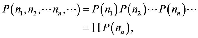(5)

which is a multi-dimensional Gaussian distribution and its maximum corresponds to each n_n being equal to, the most probable value (which is also the mean value). Again, the appropriate condition for this probability being maximum is specified by

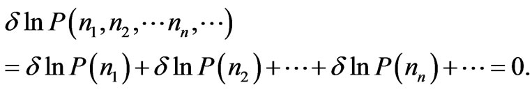(6)

When we consider the random sequences of states of the systems at a large number of instants of time, the random sequence corresponding to each instant would be characterized by one set of n_n values. Since’s are the most probable numbers, the number of random sequences having the set of values should be larger than the number of those having any other set of possible n_n values. Now we estimate the number of such sequences (having the set of values). Let S₁, S₂, , S_N0 be the sequence of particles of the assembly in some order. Each distribution of N₀ number of energy states in this sequence of N₀ number of particles leads to one sequence of energy states of the particles; there are N₀! number of such sequences. But all of them are not distinct because the same states occur many times. For instance, in any sequence the energy states between E₁ and E₁ + dE would occur number of times and permutation of these states among themselves does not lead to a new sequence of states; this is so with respect to each of the other states as well. So the total number of distinct sequences of states with number of particles in the energy states between E₁ and E₁ + dE, between E₂ and E₂ + dE, , between E_n and E_n + dE, is given by

(7)

Since’s are the most probable numbers of particles in the relevant states, the number is larger than the number N corresponding to any other set of n_n values; the subscript m denotes this. So this number should be proportional to which is the most probable value of the probability (5). Since it is appropriate to express the equilibrium condition in terms of lnP_m (rather than P_m), let us consider ln. We have from (7)

(8)

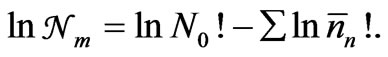
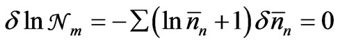
Using the Sterling approximation for the factorial of a large number n, given by lnn! = n lnn – n, (8) may be put as

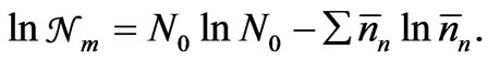(9)

Thus we see that each of the following three conditions characterize the (same) equilibrium state of the statistical assembly. When each n_n assumes its most probable value: 1) the probability P(n₁, n₂, , n_n,) has its maximum value P(), 2) the number has its largest value, and 3) the quantity has its minimum value.

In statistical physics we are interested in properties which can be attributed to an assembly over a time scale which is large compared to the time scale relevant to transitions in the “states” of the constituent systems. Such properties depend on (the physical properties relevant to) the possible states of the systems and on the probabilities associated with these states. As mentioned before the states are determined (for the systems of the given assembly) by the laws of physics, and the probabilities (or equivalently the most probable numbers of systems in different states) are to be determined by using the laws of probability (consistent, of course, with the basic properties of the assembly under consideration).

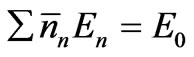
We recognize that the two basic properties of the assembly of particles under consideration are that the total number N₀ and the total energy E₀ of the particles remain constant at all instants of time. Since the most probable numbers’s are also one set of possible numbers n_n’s,

(10a)

and

. (10b)

Thus’s should satisfy the three conditions given in (9) and (10). Now being the largest number, and N₀ and E₀ being constants, we have

; (11)

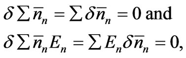(12)

where’s are small deviations from the equilibrium values’s. These three conditions should be satisfied simultaneously. Using Lagrange’s method of undetermined multipliers, we may express them as a single equation. We have

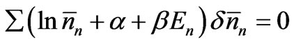, (13)

where a and b are constants. Since (13) is to be satisfied for any arbitrary set of’s, we should have

, (14)

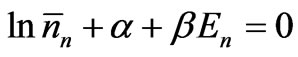
which means that

. (15)

Here is the most probable, as well as the mean, number of particles in the energy range between E_n and E_n + dE. Using the well-known arguments we may identify the constant b as 1/kT, where k is the Boltzmann constant and T the thermodynamic temperature. By virtue of (10a), a can be expressed in terms of other quantities as Z = N₀ exp a = exp (–E_n/kT); Z is called the partition function. Thus we arrive at the Maxwell-Boltzmann distribution law for energy.

4. The Conventional Approach and the New Approach

The development of statistical physics has been reviewed by Lebowitz [8]. Here we compare the distinctive features of the conventional approach (CA) and the new approach (NA). In CA [2] the object of our study is N₀ number of identical particles confined within a macroscopic volume of space; we refer to it as a many-particle system. The “state” of the many-particle system at any instant of time is specified by the position and momentum of the particles at that instant and changes continuously as a function of time as governed by (deterministic) laws of classical mechanics; the many-particle system per se is not regarded as being in statistical equilibrium. Because of the difficulties in determining the exact state of this many-particle system (due to “our incomplete knowledge” of the system), statistical approach is adopted. This conventional approach is based on three basic assumptions. 1) First we select (rather mentally) a large number of identical many-particle systems (which have “the same structure as the one of actual interest” and “are selected in such a manner as to agree with our partial knowledge as to the precise state of the actual system of interest”, and) which exist in all the different accessible states; these are said to form a “representative ensemble” of many-particle systems. The concept of ensemble is the most distinctive feature of CA [9]. 2) Next, the time-averaged values of physical quantities relevant to the actual many-particle system of our interest are assumed to be the same as the respective values averaged, at one instant of time, over the states of the many-particle systems of the ensemble. This is known as the ergodic hypothesis. 3) In taking the average over the accessible states of the many-particle systems of the ensemble, the same “weight” is given to all the states; this is the assumption of equal a priori probabilities. All the physical reasoning and mathematical derivations refer to the representative ensemble of many-particle systems. In this approach probability refers to a (many-particle) system selected at random from among an ensemble of (many-particle) systems; this is consistent with the notion of probability prevalent at the beginning of the last century.

In the new approach also our object of study is N₀ number of identical particles confined within a macroscopic volume of space; we refer to it as an assembly of many particles. The main features of the present approach are: 1) We do accept (following classical mechanics) that the “state” of an assembly of particles is specified by the position and  momentum of the particles, but in recognition of the statistical properties being independent of where the particles exist within the assembly, we specify the “state” by momentum of the particles only. 2) At the outset we recognize that collisions induce repeated transitions in the dynamical states of the particles and the assembly per se is identified as being in statistical equilibrium. All the physical reasoning and mathematical derivations refer to this assembly (only). 3) Though collision between two particles is strictly governed by deterministic laws of classical mechanics, when we consider the momentum states of the particles of the assembly (at any instant of time) in any systematic spatial order, they lead to a random sequence of these possible states. This justifies introduction of the concepts of randomness and probability into the theory (within the conceptual framework of classical determinism). 4) Probability of a state is identified as the relative frequency of the state in a random sequence of possible states. 5) The mean number of particles in the assembly having energy between E_n and E_n + dE, is shown to be the same as the most probable number of particles having energy in that range. The values of physical quantities relevant to a statistical assembly in equilibrium depend on the (time-averaged time-independent) mean numbers of particles in the various energy states, whereas the condition for statistical equilibrium is specified in terms of the most probable numbers of particles in these energy states. If the theory is to be regarded as being logically consistent, these two sets of numbers should be shown to be equal. In the present approach this has been achieved by using the central limit theorem of the probability theory. 6) The mean value of a physical quantity taken over the states of the particles in the assembly at any one instant of time, is shown to be approximately the same as the mean value taken over the different states of any single particle of the assembly at equally large number of instants of time. 7) The reason for maximizing ln () is justified, and not just accepted as a matter of convenience. In fact, only as a result of maximizing ln (instead of maximizing) do we get the exponential function in (15). A little reflection would show that maximizing ln as a matter of convenience is tantamount to assuming what is to be derived. And 8) it is shown that the minimum possible value of the quantity given by (also) specifies the equilibrium condition of the assembly. This is “Boltzmann’s famous H-theorem” which, according to Tolman, “may be regarded as among the greatest achievements of physical science”.

5. Concluding Remarks

In conclusion we may state that by making use of the modern theory of probability and statistics, it is possible to develop a new approach which is free from the concept of ensemble, the ergodic hypothesis, and the assumption of equal a priori probabilities (of the conventional approach). However, this is only an alternative approach which leads to the same final results as the well established conventional approach.

REFERENCES

- J. W. Gibbs, “Elementary Principles of Statistical Mechanics,” Dever, New York, 1960 (Reprint of 1902 Edition).
- R. C. Tolman, “The Principles of Statistical Mechanics,” Oxford University Press, Oxford, 1938.
- D. Ter Haar, “Foundations of Statistical Mechanics,” Reviews of Modern Physics, Vol. 27, No. 3, 1955, pp. 289- 338. doi:10.1103/RevModPhys.27.289
- D. Chandler, “Introduction to Modern Statistical Mechanics,” Oxford University Press, Oxford, 1987.
- R. von Mises, “Mathematical Theory of Probability and Statistics,” Academic Press, Waltham, 1964.
- M. R. Spigel, “Theory and Problems of Probability and Statistics,” McGraw-Hill, New York, 1992.
- R. Frigg, “Typicality and the Approach to Equilibrium in Boltzmann Statistical Mechanics,” Philosophy of Science, Vol. 76, No. 5, December 2009, pp. 997-1008.
- J. L. Lebowitz, “Statistical Mechanics,” In: H. Stroke, Ed., The First Hundred Years, The Physical Review, AJP Publication, New York, 1995, pp. 465-471.
- H. O. Georgii, “The Equivalence of Ensembles for Classical Systems of Particles,” Journal of Statistical Physics, Vol. 80, No. 5-6, 1995, pp. 1341-1378. doi:10.1007/BF02179874