Applied Mathematics
Vol.07 No.08(2016), Article ID:66632,12 pages
10.4236/am.2016.78068
Bayesian Posterior Predictive Probability Happiness
Gabriela Rodríguez-Hernández, Galileo Domínguez-Zacarías*, Carlos Juárez Lugo
Universidad Autónoma del Estado de México, Ecatepec, Mexico

Copyright © 2016 by authors and Scientific Research Publishing Inc.
This work is licensed under the Creative Commons Attribution International License (CC BY).
http://creativecommons.org/licenses/by/4.0/


Received 15 March 2016; accepted 17 May 2016; published 20 May 2016
ABSTRACT
We propose to determine the underlying causal structure of the elements of happiness from a set of empirically obtained data based on Bayesian. We consider the proposal to study happiness as a multidimensional construct which converges four dimensions with two different Bayesian techniques, in the first we use the Bonferroni correction to estimate the mean multiple comparisons, on this basis it is that we use the function t and a z-test, in both cases the results do not vary, so it is decided to present only those shown by the t test. In the Bayesian Multiple Linear Regression, we prove that happiness can be explained through three dimensions. The technical numerical used is MCMC, of four samples. The results show that the sample has not atypical behavior too and that suitable modifications can be described through a test. Another interesting result obtained is that the predictive probability for the case of sense positive of life and personal fulfillment dimensions exhibit a non-uniform variation.
Keywords:
Bayesian Inference, Posterior Predictive Distribution, MCMC, Happiness

1. Introduction
Bayesian networks emerged about three decades ago as alternatives to conventional systems-oriented decision- making and forecasting under uncertainty in probabilistic terms [1] . A Bayesian network is a statistical tool that represents a set of associated uncertainties given conditional independence relationships established between them [2] [3] .
The rule Bayes is a rigorous method for interpreting evidence in the context of previous experience or knowledge. The Bayes rule has recently emerged as a powerful tool with a wide range to applications which include: genetics, image processing, ecology, physics and engineering. The essential characteristics of Bayesian methods are their explicit use of probability for quantifying uncertainty in inferences base on statistical data analysis. A Bayesian probability interval for an unknown quantity of interest can be directly regarded as having a high probability of containing the unknown quantity, in contrast to a frequentist confidence interval which may strictly be interpreted only in relation to a sequence of similar inferences that might be made in repeated practice.
Using Bayesian networks as a tool for data analysis is not widespread in the context of Psychology. However, the benefits of using this tool in all areas of psychology are identified in several ways: on the economic front with Bayesian networks could develop systems to make judgments appropriate chance to improve diagnosis and psychological treatment. On the scientific level, Bayesian networks cannot be overlooked if psychology strives to clarify the mechanisms by which people evaluate, decide and make inferences; as they may serve as analytical and theoretical reference in the development of models of reasoning, learning and perception of uncertainty [3] .
In psychology, the area’s most prolific work in the use of Bayesian networks has been the causal learning [4] - [7] , where they test the hypothesis that people represent causal knowledge similarly to as it does a Bayesian network. Other theoretical developments have made possible to extend the use of Bayesian network outside the domain of causal knowledge, for instance, on inductive generalization of concepts and learning words [8] . Another facet of Bayesian networks which have proved useful tools is in market research [9] . Others found that a Bayesian network classifies customers of a company relative to the perspective of long-term purchases [10] . On the other hand, it analyzed the nature of human emotions and the negative behavior resulting from overcrowding during mass events. Utilizing the Bayesian network, his model shows the dependence structure between different emotions and negative behaviors of pilgrims in the crowd [11] .
Finally, by its shaping power, the Bayesian networks could be used to generate more and better models of how organizations, groups or social aggregate which is the subject of study for psychology. Thus the aim of this study was to determine the underlying causal structure of the elements of happiness from a set of empirically obtained data. It is considered a Bayesian statistical parameter, which is inferred as an uncertain event, in this study the knowledge about happiness is not accurate and is subject to uncertainty, therefore happiness can be described by a probability distribution. Whereby the Metropolis algorithm used is a specific type of process Monte Carlo, which generates a random way so that every step along the way is completely independent of the previous steps of the current position and generates Markov chains. Process in each step has not memory of the previous states. This is known as Markov Chain Monte Carlo (MCMC)
Happiness has been defined as an entity that can be described by a specific set of measures [12] , [13] , a mental state that people can gain control over in a cognitive way to perceive and conceive both themselves and their world as an experience of joy, satisfaction or positive welfare [14] . Unfortunately, terms like happiness have been used frequently in daily discourse and may now have vague and somewhat different meanings.
The difficulty of defining happiness has led pioneer psychologists in the study of happiness propose the term subjective well-being (SWB). SWB refers to people's evaluations of their own lives and encompasses both cognitive judgments of satisfaction and affective appraisals of moods and emotions. This conceptualization emphasizes the subjective nature of happiness and holds individual human beings to be the best judges of their own happiness [15] - [17] .
There is empirical evidence indicating that well-being is a much broader construct than stability of emotions and subjective judgment about life satisfaction; e.g. situational models consider that the sum of happy moments in life results in the satisfaction of people [18] , that is, a person exposed to a greater amount of happy events will be more satisfied with his or her life. People briefly react to good and bad events, but in a short time they return to neutrality. Thus, happiness and unhappiness are merely short-lived reactions to changes in people [19] and it depends strongly on intentional activity [20] , [21] . But also it has been identified the temperament is suggested to influence happiness [22] , [23] and other personality traits such as optimism and self-esteem [24] - [26] , the self-determination [27] .
Scholars have noticed that happiness is not a single thing, but it can be broken down into its constituent elements. Considering this information, Alarcón [28] proposes to study happiness as a multidimensional construct which converges satisfaction of what has been achieved, positive attitudes toward life, (experiences that reflect positive feelings concerning one’s self and life) personal fulfillment, and joy of living.
Happiness Scale of Lima (HSL) [28] , consists of 27 items and reported item-scale correlations were highly significant and high internal consistency (∝ = 0.92). The factorial analysis of principal components and varimax
rotation, revealed that happiness is a multidimensional behavior, consisting of four dimension:  Sense positive of life,
  Satisfaction with life,
  Personal fulfillment and
  Joy of living.
2. The Model
Definition 1
The σ-algebra is used for measured definition. A probability measure is a mapping  that assigns a probability
  to any event, with the properties
  and
and  whenever
 . A real value random variable is a mapping
  and
and 
Definition 2
A random variables es given by  where is measurable and subset of
 , we denote by
  then the event is
 .
.
Definition 3
The random samples, say ,
,  ,
,  y
y , have the same underlying distribution.
We assume that we have four data samples . If the data have the same distributions, then
 . Uncertainty about the true value of parameter it described by a measurement conditional observed datasets. The posterior predictive distribution, is defined as
 (1)
(1)
Lema 1.
Let  be a probability measure on
  such that

The probability for  denoted
  is equal to the joint probability
  for any fixed
 , the probability is bounded by
 (2)
(2)
Consider the problem of selecting independent samples from several populations for the purpose of between-group comparisons, either through hypothesis testing or estimation of mean differences. A companion problem is the estimation of within-group mean levels. Together, these problems form the foundation for the very common analysis of variance framework, but also describe essential aspects of stratified sampling, cluster analysis, empirical Bayes, and other settings. Procedures for making between-group comparisons are known as multiple comparisons methods. The goal of determining which groups have equal means requires testing a collection of related hypotheses [29] .
Consider independent samples from l normally distributed populations with equal variances (3a y 3b)
 (3a)
(3a)
 (3b)
(3b)
Then  for each
  then there is
  tests. For example, for two sample there is 1 test, for three sample there is 3 test, and 4 there is 6 test. When two or more means are taken as equal, we merely combine all relevant samples into one.
Let  denote the observed data. Assume that
  is to be described using a model
  selected from a set of candidate models
 . Assume that each
  is uniquely parameterized by
 , an element of the parameter space
 . In the multiple comparisons problem, the class of candidate models consists of all possible mean level clustering. Each candidate model is parameterized by the mean vector
  and the common variance
 , with the individual means restricted by the model defined clustering of equalities. That is, each model determines a corresponding parameter space where particular means are taken as equal.
Let , where
  take values in a d-dimensional parameter space
 , be likelihood [30] - [33] functions associated with the samples and
  denote a prior density on
  over the model
 . Then
  denote a prior on
  given the model
 . The posterior probability for
  and
and  can be written as
 (4)
(4)
 (5)
(5)
You can write the posterior probability (4) y (5) as,
 (6)
(6)
We use a uniform prior for  (6) it can be written as


we using equations (5,6) and the previous development, we write the following relationship
 (7)
(7)
Definition 4
The Taylor series of a real or complex-valued function  that is infinitely differentiable at a real or complex number is the power series

Then, applying the definition 4 to (7), we obtain
 (8)
(8)
The Fisher information [30] is a way of measuring the amount of information that an observable random variable X carries out unknown parameter θ.
 (9)
(9)
Applying (9) to (8), is obtained

 (10)
(10)
taken


Then
 (11)
(11)
With respect to the candidate model class , we obtain, the posterior model probabilities
 (12)
(12)
Many clever methods have been devised for constructing and sampling from arbitrary posterior distributions. Markov chain simulation (also called Markov chain Monte Carlo, or MCMC) is a general method based on drawing values of θ from approximate distributions and then correcting those draws to better approximate the
target posterior distribution,  [34] [35] . The sampling is done sequentially, with the distribution of the sampled draws depending on the last value drawn; hence, the draws form a Markov chain. (As defined in probability theory, a Markov chain is a sequence of random variables
  for which, for any t, the distribution
of  given all previous θ’s depends only on the most recent value) The key to the method’s success, however, is not the Markov property but rather that the approximate distributions are improved at each step in the simulation, in the sense of converging to the target distribution [35] .
A z-statistic should be calculated when the standard deviation of the population(s) is known. If the standard deviation is not known, then the standard error must be estimated using the standard deviation of the sample(s). Due to this estimation, we must use the t-distribution which is thicker in the tails to account for estimating the standard error with the sample standard deviation [34] .
 (13)
(13)
 (14)
(14)
Until now, we have built the theory to apply to the case of four sample data, now what we will do, will be a particular case study, and see that Lema and definitions 1, 2 y 3 are applied naturally like the Equation (14)
Example particular case
Suppose . Select a random sample of size
 . From ith group
  so sample sizes are

 is the sample mean for the observations in all group combined


Variability in the data, the deviation of an individual observation


To test the null hypothesis that the population means are all the same, us the test statistic

Under , this statistic has t distribution with k-1 and n-k degree freedom.
Now four three
Suppose . Select a random sample of size ni. From ith group
  so sample sizes are


Then 

and


The principle of Bayes model is to compute posteriors bases on specified priors and the likelihood function of data, the four groups of size 1110.
We began with a descriptive model of data from four groups, wherein the parameters were meaningful measures of central tendency, variance, and normality. Bayesian inference reallocates credibility to parameter values that are consistent with the observed data. The posterior distribution across the parameter values gives complete information about which combinations of parameter values are credible. In particular, from the posterior distribution we can assess the credibility of specific values of interest, such as zero difference between means, or zero difference between standard deviations. We can also decide whether credible values of the difference of means are practically equivalent to zero, so that we accept the null value for practical purposes.
The Bayesian posterior distribution can also be used as a complete hypothesis for assessing power, that is, the probabilities of achieving research goals such as rejecting a null value, accepting a null value, or reaching a desired precision of estimation. The power estimation incorporates all the information in the posterior distribution by integrating across the credible parameter values, using each parameter-value combination to the extent it is credible. Figure 1 shows histograms of data that are labeled with  on their abscissas, and these data are fixed at their empirically observed values.
3. Bayesian Multiple Linear Regression
 now, we need to find an adjustment function for the above data. A linear regression model where more than one variable involved is called multiple regression model [36] - [38]
 (15)
(15)
where, we have k regressors, parameters  they are regression coefficients, then the Approach Bayesian Multiple Linear Regression is [36] [37]
 (16)
(16)
The prior distribution of  is NIG (Normal-Inverse-Gamma) and it is given by
  thus
thus  they are hyperparameters.
 (17)
(17)


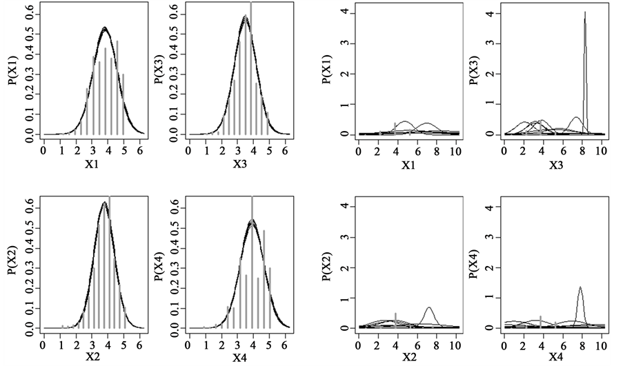
Figure 1. Posterior predictive probability dimensions.

where IG (Inverse Gaussian)
If we denote by  y
y 
We can express the density function as
 (18)
(18)
The conjugate prior distribution will be given by
 (19)
(19)
In the scheme MCMC
 (20)
(20)
where  is a matrix (n ´ p) and
  is the covariance matrix and
  is a vector dimension p of regression coefficients to do Bayesian estimation. Assume the prior distribution of
  is
is
 (21)
(21)
where  and
and  are matrices representing our beliefs about average and covariance of prior distribution. Take
  and using Bayesian approach, we obtain
 (22)
(22)
where


We can see that both matrices have two terms, one that only it depends on the prior and other that only it depends of data. This is very useful because in each iteration. We have to update only the last term. The question to be dealt is the choice of hyperparameters  y
y 


Then, we can write the equation as follows [38]
 (23)
(23)
Figures 2-5 show the range HDI, which means Higher Density Interval. Values inside HDI have a greater probability density (credibility) that values outside this. Therefore, the 95% HDI includes the most incredible parameters values. There is a way that the posterior 95% HDI could exclude zero even when the data have a frequency of zero. It can happen if the prior already excludes zero. This interval is useful as a summary of the distribution and decision tool. The decision rule is simple. Any value outside of the 95% HDI is rejected [38] .
In all four cases the focus is on assessing if the predictors were differentially predictive, for which we examine the posterior distribution of the differences standardized regression coefficients, given that the comparison is based in the normalization using the single sample.
As shown in Figure 2, the data to  none of the coefficients are within the supposed. We observed than for X1 (sense positive of life) for differences in
  are out of interval to be credible, indicating than
 , cannot be a linear combination of the other dimensions.
In Figure 4, the outcomes for dataset  where X2 (satisfaction with life)
 ,
,
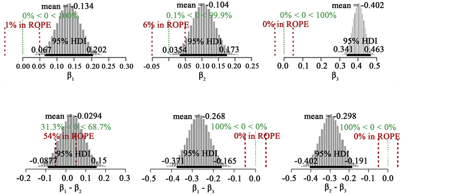
Figure 2. Posteriori distribution for X1.
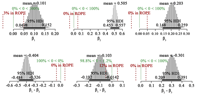
Figure 3. Posteriori distribution for X2.
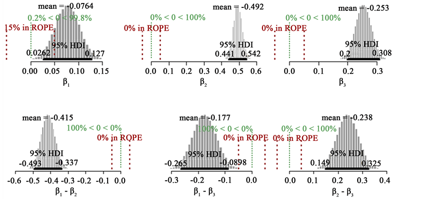
Figure 4. Posteriori distribution for X3.
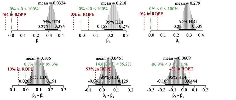
Figure 5. Posteriori distribution for X4.
HDI goes from 0.209 to 0.391. Therefore X1 and X3 are equally costly and if we want to avoid double cost of measuring both, then, is probable to be more effective assess X2 than X3.
In Figure 5 the outcomes for dataset , where X3 (personal fulfillment)
 ,
,
HDI goes from 0.149 to 0.325. Therefore X1 and X2 are equally costly and if we want to avoid double cost of measuring both, then, is probable to be more effective assess X1 than X4.
Figure 5 shows for dataset , where X4 (joy of living)
 , HDI goes from
0.0205 to 0.191. Therefore X1 and X2 are equally costly, and if we want to avoid double cost of measuring both, then, is probable to be more effective assess X1 than X2.
The template is used to format your paper and style the text. All margins, column widths, line spaces, and text fonts are prescribed; please do not alter them. You may note peculiarities. For example, the head margin in this template measures proportionately more than is customary. This measurement and others are deliberate, using specifications that anticipate your paper as one part of the entire journals, and not as an independent document. Please do not revise any of the current designations.
4. Conclusions
Bayesian methods have been developed as a tool for reasoning quantitatively in situations where arguments cannot be made with certainty. The focus recent developments of Markov chain Monte Carlo algorithms, in many situations the only way to integrate over the parameter space. The use of posterior predictive distributions makes the method robust to the choice of priors on the model parameters and enables the use of improper priors even when only very few observations are available. To measure the agreement between posterior predictive distributions, we derive a measure which has an intuitive probabilistic interpretation.
Within the discussion of the results, we found that the sample has not atypical behavior, too, and that suitable modifications can be described through a test. Another interesting result obtained is that the predictive probability for the case of X1 (sense positive of life) and X3 (personal fulfillment) dimensions exhibit a non-uniform variation, while other factors are uniform distribute.
The hypotheses of work, was that if through sample analysis could infer that happiness, only one is affected by three dimensions X2 (sense positive of life), X3 (personal fulfillment) and X4 (satisfaction with life). In this context, we note that the hypothesis was tested, the marked tendency on distributions in recent factors was sufficient to support this theory, on the other hand, through the Multilinear Regression Bayesian, also tested this hypothesis.
Due to recent revolutionary advances in Bayesian posterior computation via computer-intensive MCMC simulation techniques, difficulties with posterior computations can be overcome. A Bayesian state-space model is readily implemented using standard Bayesian software such as JAGS, BUGS, NIMBLE and STAN. One can therefore avoid writing one-off programs in a low-level language. Any modifications, such as different prior distributions, applications to different data sets, or the use of different sampling distributions, require the change of just a single line in the code.
Cite this paper
Gabriela Rodríguez-Hernández,Galileo Domínguez-Zacarías,Carlos Juárez Lugo, (2016) Bayesian Posterior Predictive Probability Happiness. Applied Mathematics,07,753-764. doi: 10.4236/am.2016.78068
References
- 1. Seligman, M., Steen, T., Park, N. and Peterson, C. (2005) Positive Psychology Progress: Empirical Validation of Interventions. American Psychologist, 60, 410-421.
http://dx.doi.org/10.1037/0003-066X.60.5.410 - 2. Lyubomirsky, S. (2008) La ciencia de la Felicidad. Un método probado para conseguir el bienestar. Ediciones Urano, Santiago.
- 3. Diener, E. (2000) Subjective Well-Being: The Science of Happiness and Proposal for a National Index. American Psychologist, 55, 34-43.
http://dx.doi.org/10.1037/0003-066X.55.1.34 - 4. Diener, E. (2009) Subjective Well-Being. In: Diener, E., Ed., The Science of Well-Being: The Collected Works of Ed Diener, Social Indicators Research Series 37, Springer Science + Bussiness Media B. V, 11-58.
http://dx.doi.org/10.1007/978-90-481-2350-6_2 - 5. Diener, E., Sandvik, E. and Pavot, W. (1991) Happiness Is the Frequency, Not the Intensity, of Positive versus Negative Affect. In: Strack, F., Argyle, M. and Schwarz, N., Eds., Subjective Well-Being: An Interdisciplinary Perspective, Pergamon, New York, 119-139.
- 6. Veenhoven, R. (1994) Is Happiness a Trait? Social Indicators Research, 32, 101-160.
http://dx.doi.org/10.1007/BF01078732 - 7. Lyubomirsky, S., Sheldon, K.M. and Schkade, D. (2005) Pursuing Happiness: The Architecture of Sustainable Change. Review of General Psychology, 9, 111-131.
http://dx.doi.org/10.1037/1089-2680.9.2.111 - 8. Sheldon, K.M. and Lyubomirsky, S. (2006) Achieving Sustainable Gains in Happiness: Change Your Actions, Not Your Circumstances. Journal of Happiness Studies, 7, 55-86.
http://dx.doi.org/10.1007/s10902-005-0868-8 - 9. Diener, E., Helliwell, F.B. and Kahneman, D. (2010) International Differences in Well-Being. Oxford University Press, New York.
http://dx.doi.org/10.1093/acprof:oso/9780199732739.001.0001 - 10. Diener, E. and Lucas, R. (2008) Personality and Subjective Well-Being. In: John, O., Robins, R. and Pervin, L., Eds., Handbook of Personality, 3rd Edition, Guilford, New York, 795-814.
- 11. Lucas, R. and Fujita, F. (2000) Factors Influencing the Relation between Extraversion and Pleasant Affect. Journal of Personality and Social Psychology, 79, 1039-1056.
- 12. Lucas, R., Diener, E. and Suh, E. (1996) Discriminant Validity of Well-Being Measures. Journal of Personality and Social Psychology, 71, 616-628.
http://dx.doi.org/10.1037/0022-3514.71.3.616 - 13. Peterson, C. (2000) The Future of Optimism. American Psychologist, 55, 44-55.
http://dx.doi.org/10.1037/0003-066X.55.1.44 - 14. Schimmack, U. and Diener, E. (2003) Predictive Validity of Explicit and Implicit Self-Esteem for Subjective Well-Being. Journal of Research in Personality, 37, 100-106.
- 15. Ryan, R.M. and Deci, E. (2000) Self-Determination Theory and the Facilitation of Intrinsic Motivation, Social Development, and Well-Being. American Psychologist, 55, 68-78.
http://dx.doi.org/10.1037/0003-066X.55.1.68 - 16. Alarcón, R. (2006) Desarrollo de una Escala Factorial para medir Felicidad. Interamerican Journal of Psychology, 40, 99-106.
- 17. Blomstedt, P., Gauriot, R., Viitala, N., Reinikainen, T. and Corander, J. (2014) Bayesian Predictive Modeling and Comparison of Oil Samples. Journal of Chemometrics, 28, 52-59.
http://dx.doi.org/10.1002/cem.2566 - 18. Yin, Y. and Li, B. (2014) Analysis of the Behrens-Fisher Problem Based on Bayesian Evidence. Journal of Applied Mathematics, 2014, Article ID: 978691.
http://dx.doi.org/10.1155/2014/978691 - 19. Myung, J.I. (2003) Tutorial on Maximum Likelihood Estimation. Journal of Mathematical Psychology, 47, 90-100.
http://dx.doi.org/10.1016/S0022-2496(02)00028-7 - 20. Mossel, E. and Tamuz, O. (2010) Iterative Maximum Likelihood on Networks. Advances in Applied Mathematics, 45, 36-49.
http://dx.doi.org/10.1016/j.aam.2009.11.004 - 21. Mengersen, K.L., Pudlo, P. and Robert, P.C. (2013) Bayesian Computation via Empirical Likelihood. Proceedings of the National Academy of Sciences of the United States of America, 110, 1321-1326.
http://dx.doi.org/10.1073/pnas.1208827110 - 22. Lensen, J.L. (1987) A Note on Asymptotic Expansions for Markov Chains Using Operator Theory. Advances in Applied Mathematics, 8, 377-392.
http://dx.doi.org/10.1016/0196-8858(87)90016-9 - 23. D’Angeli, D. and Donno, A. (2013) The Lumpability Property for a Family of Markov Chains on Poset Block Structures. Advances in Applied Mathematics, 51, 367-391.
http://dx.doi.org/10.1016/j.aam.2013.04.007 - 24. Mitchell, T.J. and Beauchamp, J.J. (1988) Bayesian Variables Selection in Linear Regression. Journal of the American Statistical Association, 83, 1023-1032.
http://dx.doi.org/10.1080/01621459.1988.10478694 - 25. Hoeting, J., Raftery, A.E. and Madigan, D. (1996) A Method for Simultaneous Variables Selection and Outlier Identification in Linear Regression. Computational Statistics & Data Analysis, 22, 251-270.
http://dx.doi.org/10.1016/0167-9473(95)00053-4 - 26. Kruschke, J.K. (2015) Doing Bayesian Data Analysis: A Tutorial with R, JAGS, and Stan. Academic Press/Elsevier, Waltham.
- 27. Seligman, M. (2011) Flourish. A Visionary New Understanding of Happiness and Well-Being. Free Press, New York.
- 28. Ramli, N., Abdul G., Ahmad, H., Mohd, H., Sulong, J., Mohd, M., Abd, R. and Mat, S. (2014) Bayesian Network Model of Crowd Emotion and Negative Behavior. AIP Conference Proceeding, 163, 867.
http://dx.doi.org/10.1063/1.4903685 - 29. Baesens, B., Verstraeten, G., Van den Poel, D., Egmont-Petersen, M., Van Kenhove, P. and Vanthienen, J. (2004) Bayesian Classifiers for Identifying the Slope of the Customer Life Cycle of Long-Life Customer. European Journal of Operational Research, 156, 508-523.
http://dx.doi.org/10.1016/S0377-2217(03)00043-2 - 30. Nadkarni, S. and Shenoy, P.P. (2001) A Bayesian Network Approach to Making inferences in Causal Maps. European Journal of Operational Research, 128, 479-498.
http://dx.doi.org/10.1016/S0377-2217(99)00368-9 - 31. Tenenbaum, J.B., Griffiths, T.L. and Kemp, C. (2006) Theory-Based Bayesian Models of Inductive Learning and Reasoning. Trends in Cognitive Science, 10, 309-318.
http://dx.doi.org/10.1016/j.tics.2006.05.009 - 32. Waldman, M.R. and Hagmayer, Y. (2005) Seeing versus Doing: Two Models of Accessing Causal Knowledge. Journal of Experimental Psychology: Learning, Memory, and Cognition, 31, 216-227.
http://dx.doi.org/10.1037/0278-7393.31.2.216 - 33. Sobel, D.M., Tenenbaum, J.B. and Gopnik, A. (2004) Children’s Causal Inferences from Indirect Evidence: Backwards Blocking and Bayesian Reasoning in Preschoolers. Journal of Experimental Psychology, 130, 380-400.
http://dx.doi.org/10.1207/s15516709cog2803_1 - 34. Gopnik, A. and Schulz, L. (2004) Mechanisms of Theory Formation in Young Children. Trends in Cognitives Sciences, 8, 371-377.
http://dx.doi.org/10.1016/j.tics.2004.06.005 - 35. Gopnik, A., Glymour, C., Sobel, D.M., Schulz, L.E., Kushnir, T. and Danks, D. (2004) A Theory of Causal Learning in Children: Causal and Bayes Nets. Psychological Review, 111, 3-32.
http://dx.doi.org/10.1037/0033-295X.111.1.3 - 36. Edwards, W. (1998) Hailfinder. Tools for and Experiences with Bayesian Normative Modelling. American Psychologist, 53, 416-428.
http://dx.doi.org/10.1037/0003-066X.53.4.416 - 37. Cowell, R.G., Dawid, A.P., Lauritzen, S.L. and Spiegelhalter, D.J. (1999) Probabilistic Networks and Expert Systems. Springer, Harrisonburg.
- 38. Pearl, J. (2001) Bayesian Networks, Causal Inference and Knowledge Discovery (Tech. Rep. R-281). University of California, Los Angeles.
NOTES

*Corresponding author.