Applied Mathematics
Vol.5 No.14(2014), Article ID:48155,13 pages
DOI:10.4236/am.2014.514205
Mixed Model, AMMI and Eberhart-Russel Comparison via Simulation on Genotype × Environment Interaction Study in Sugarcane
Guilherme Moraes Ferraudo1, Dilermando Perecin2
1CanaVialis/Monsanto, Campinas, Brazil
2Departamento de Ciências Exatas, Faculdade de Ciências Agrárias e Veterinárias, UNESP—Universidade Estadual Paulista, Campus Jaboticabal, Jaboticabal, Brazil
Email: gferrau@monsanto.com, perecin@fcav.unesp.br
Copyright © 2014 by authors and Scientific Research Publishing Inc.
This work is licensed under the Creative Commons Attribution International License (CC BY).
http://creativecommons.org/licenses/by/4.0/


Received 5 May 2014; revised 10 June 2014; accepted 20 June 2014
ABSTRACT
Brazil is the world leader in sugarcane production and the largest sugar exporter. Developing new varieties is one of the main factors that contribute to yield increase. In order to select the best genotypes, during the final selection stage, varieties are tested in different environments (locations and years), and breeders need to estimate the phenotypic performance for main traits such as tons of cane yield per hectare (TCH) considering the genotype × environment interaction (GEI) effect. Geneticists and biometricians have used different methods and there is no clear consensus of the best method. In this study, we present a comparison of three methods, viz. Eberhart-Russel (ER), additive main effects and multiplicative interaction (AMMI) and mixed model (REML/BLUP), in a simulation study performed in the R computing environment to verify the effectiveness of each method in detecting GEI, and assess the particularities of each method from a statistical standpoint. In total, 63 cases representing different conditions were simulated, generating more than 34 million data points for analysis by each of the three methods. The results show that each method detects GEI differently in a different way, and each has some limitations. All three methods detected GEI effectively, but the mixed model showed higher sensitivity. When applying the GEI analysis, firstly it is important to verify the assumptions inherent in each method and these limitations should be taken into account when choosing the method to be used.
Keywords:Plant Breeding, Data Simulation, Genotype-Environment Interaction (GEI) Detection Methods, R Computing Environment, REML/BLUP

1. Introduction
Sugarcane produces energy and food for the world and the sugarcane sector plays a very important role in the Brazilian agribusiness. Currently, Brazil is the world’s largest sugar exporter.
Reference [1] used data from trials conducted at Agronomic Institute (IAC) Sugarcane Center, Brazil, and showed that, between 1994-2006, genetic gain provided increases of 1.25 tons of cane yield per hectare per year (TCH) (1.16% yearly for TCH and 1.28% yearly for tons of sucrose yield per hectare (TPH)) in the plant cane (first harvest). In the first ratoon (second harvest), gains reached 0.59% yearly for TCH and 1.43% yearly for TPH. Yield increase is attributed to several factors and the development of new sugarcane cultivars stands out as one of the main aspects, highlighting the importance of the plant breeding for the sugarcane.
In the final stages of selection in breeding programs, where there is a great amount of material available for each advanced genotype, it is possible to characterize genotypes in terms of genotype × environment interaction (GEI). The genotypes are planted in different environments (locations and years) to identify the best genotype, based on phenotypic performance of interest such as TCH, which is the main trait to measure sugarcane yield. For the breeder, understanding the aspects that affect GEI is essential to implement an efficient selection process and to select sites for evaluation [2] .
The complexity of GEI makes it difficult for breeders to recommend superior genotypes as it is a field of research with plenty of room for further studies. Various methods have been used to evaluate GEI in different crops, however there is no consensus regarding the best method to be used. Reference [3] reported that GEI has been the object of research of biometricians and quantitative geneticists since the beginning of the 20th century and a number of stability indices have been developed to quantify and select genotypes taking into account GEI. Among the main methods used to evaluate GEI, the following can be highlighted: 1) Eberhart-Russel (ER) [4] ; 2) Additive main effects and multiplicative interaction (AMMI) [5] -[12] ; and 3) mixed model [13] -[16] . The literature shows several studies on the use of these three methods to assess GEI in sugarcane [2] [17] -[20] as well as in other crops [21] -[25] . However, no studies containing simulations comparing the three methods (ER, AMMI and mixed model) have been reported.
Therefore, because of the different scenarios obtained from the simulation data, the objectives of this study were: 1) to determine the efficiency of each method (ER, AMMI and mixed model) in detecting GEI; and 2) to discuss the specificities of the methods.
2. Materials and Methods
2.1. Simulation Data
Initially, 1000 trials (replicas, in the terminology of simulation studies) were simulated containing 15 genotypes in 12 environments and within each environment, three replications (blocks), according to the method of analysis of experiments following the randomized complete block design (RCBD) for each environment. The trait (response variable) simulated was TCH, which is used to measure sugarcane yield. All the simulation conditions aimed to represent the different practical situations inherent in experiments of breeding programs for sugarcane.
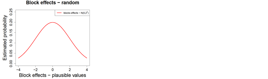
The block effects were generated from a Normal probability distribution with zero mean and standard deviation equal to two, that is, N(0,22). The effects of the twelve environments were generated from the following Normal probability distributions: Env1 ~ N(−20,42); Env2 ~ N(−10,42); Env3 ~ N(−5,42); Env4 ~ N(−2,42); Env5 ~ N(0,42); Env6 ~ N(0,42); Env7 ~ N(0,42); Env8 ~ N(0,42); Env9 ~ N(2,42); Env10 ~ N(5,42); Env11 ~ N(10,42); Env12 ~ N(20,42). A systematic variation is observed from -20 to +20 for the mean. The null effect was considered in four environments, and the standard deviation for the twelve environments was fixed and equal to 4 t∙ha−1. The Normal probability distributions to the block and environment effects are shown in Figure 1.
The genotypes formed three groups based on the average yield and the corresponding Normal probability distributions for each of the three simulation scenarios: 1) simulation scenario 1—random and coefficient of variation equals to 5% (RCV); 2) simulation scenario 2—random and standard deviation equals to 8 t∙ha−1 (RSD); and 3) simulation scenario 3—ystematic and standard deviation equals to 8 t∙ha−1 (SySD) are shown in Table 1 and Figure 2.
All simulations of such effects followed the Normal probability distribution, and the simulations were independent from one another. In the Normal probability distributions, the mean was dependent on the genotype condition, the block effect and the environment.

Table 1. Normal probability distributions to simulate the effects of each genotype for the different genotypes groups and simulation scenarios.
 (a)
(a)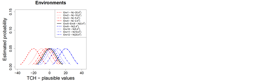 (b)
(b)
Figure 1. Normal theoretical probability distributions to the block simulated effects (a) and environments (b).
 (a)
(a)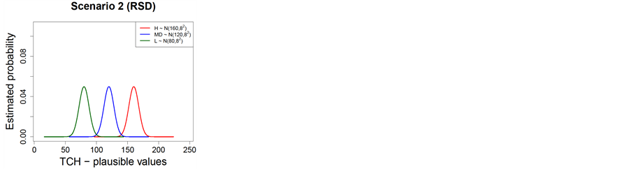 (b)
(b)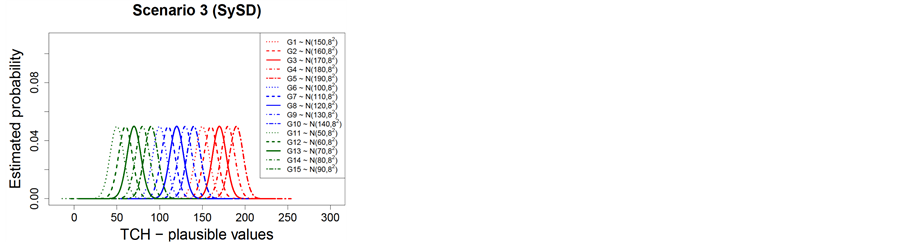 (c)
(c)
Figure 2. Normal theoretical probability distributions for the different genotypes groups and simulation scenarios (Scenario 1—RCV (a); Scenario 2—RSD (b); Scenario 3—SySD (c)).
In RCV, the increase in the mean (location parameter) is accompanied by the increase of the variance (scale parameter) of the data, meaning that the smaller the mean, the lower the data variability. In other words, the mean and the variability of group of genotype H are greater than the average and the variability of group MD, which, in turn, are greater than the mean and the variability of group L.
Distribution in group L is well-concentrated (low variability) around the mean. There is overlap of distributions with the same mean and variance within each group of genotype (H, MD and L). RCV is the only simulation scenario that shows heterogeneity of variance among the genotypes groups.
For RSD, there is displacement of the mean in the distributions, however, the variance remains constant (homogeneity of variance). Again, there is overlap of distributions within each genotype group (H, MD and L). For SySD, there is greater displacement of the mean in distributions when compared to distributions in RCV and RSD scenarios, however, the variance remains constant in SySD as well as in RSD. In SySD, there is no overlap of distributions with the same mean and variance within each group of genotype (H, MD and L); however, it shows a larger number of distributions with different means within each genotype group. This displacement of distributions is due to the systematic addition over the mean condition of each genotype within each genotype group (H, MD and L), indicating that there is genotypic effect within each genotypes group.
Nevertheless, the simulation data in accordance with the conditions in each scenario through the described pseudo-random distributions do not show GEI. Thus, there would be no conditions to ensure that the objectives of this work could be achieved. Therefore, it was necessary to add (force) GEI to the simulation conditions. GEI was created by exchanging (inversion) the responses between the genotypes of different groups (H, MD and L), varying the environments where GEI occurred.
The following strategies were used to assess the inversions:
1. EG_1HMD: inversion of a genotype of high yield (H) with one of medium yield (MD);
2. EG_1HL: inversion of an H genotype with a genotype of low yield (L);
3. EG_1MDL: inversion of an MD with an L genotype;
4. EG_2HMD: inversion of two H with two MD genotypes;
5. EG_2HL: inversion of two H with two L genotypes;
6. EG_2MDL: inversion of two MD with two L genotypes;
7. EG_3HMD: inversion of three H with three MD genotypes;
8. EG_3HL: inversion of three H with three L genotypes;
9. EG_3MDL: inversion of three MD with three L genotypes.
The genotypes inversion was performed by exchanging the names of genotypes considering the three groups of environments: 1) within the neutral environments (E1): Env5, Env6, Env7 and Env8; 2) between the worst and the best environments (E2): when the exchange involved two genotypes belonging to different groups of genotypes, the inversion was made between the groups of environments—Env1, Env2, Env3 and Env4 versus Env9, Env10, Env11 and Env12 versus Env1 and Env12; and 3) unstructured exchanges within each group of environments (E3): this type of exchange aimed to accomplish more complex interactions. When the exchange involved two genotypes belonging to different groups of genotypes, the inversion was made between the groups of environments—Env1, Env2, Env8, Env10 and Env12 versus Env3, Env9 and Env11; and, when the exchange involved three genotypes, belonging to different groups, the inversion was carried out between the groups of environments—Env1, Env2, Env8, Env10 and Env12 versus Env3, Env9 and Env11 versus Env1, Env4, Env6 and Env12.
In this manner all the situations that led to the construction of the final simulation cases were created. Genotypes had three scenarios (Table 1). Blocks had a single scenario-random zero mean and standard deviation equal to 2. Three groups of environments were created (E1, E2 and E3), where the exchanges were evaluated. Within group E1, we made all exchanges evaluated, from one to three exchanges of genotypes among the genotypes groups (H, MD and L), totaling 27 cases. Within groups E2 and E3, we carried out exchanges between two and three genotypes, totaling 18 exchanges in E2 and 18, in E3. Adding all the cases (27 in E1 + 18 in E2 + 18 in E3), we obtained the 63 final cases that were simulated and will be discussed below. The first five columns of Table 2 refer to the cases, the number of exchanges carried out, the group of environments where the exchanges were made, the abbreviations of each simulation scenario and the type of exchange between genotypes and the exchange that was introduced in each case. These columns aim to clarify the procedures carried out in each simulation case.
Table 2 .Percentage of statistical significance (p-value < 0.05) of GEI for the following statistics: F of GEI in usual univariate ANOVA; regression deviations in ER; scores of genotypes in AMMI outside the confidence interval (AMMI1) or the confidence region (AMMI2 or AMMI3); t associated to BLUPs of GEI effects for genotypes that were exchanged in environments where exchanges occurred (BLUP GenCEnvC); t associated to BLUPs of GEI effects for genotypes that were exchanged in environments where no exchanges occurred (BLUP GenCEnvNC) and t associated to BLUPs of GEI effects for genotypes that did not undergo any type of exchange in all environments (BLUP GenNC) in each simulation case.
Therefore, each of the 63 simulation cases shows a sampling distribution of the particular TCH values due to the different conditions and exchanges described in this section. The data are balanced and there is no correlation structure between the effects.
In total, 63 cases were evaluated and for each case, we simulated 540 observations (15 genotypes × 12 environments × 3 replications = 540) and 1,000 replicas and each case was analyzed by the three methods. Thus, each of the three methods evaluated 34,020,000 data points (540 observations × 1000 replicas × 63 cases = 34,020,000).
2.2. GEI Evaluation Methods
In this study the following methods were used: 1) ER; 2) AMMI; and 3) mixed model (restricted maximum likelihood (REML)/best linear unbiased prediction (BLUP)).
2.2.1. The ER Method
The use of linear regression to identify stable genotypes was initially proposed by [26] . The authors proposed separating GEI into a multiplicative term and a deviation to verify whether GEI is a linear function of the additive environmental component.
In theory, a sufficient condition for linear regression is that the joint distribution
of yield and the environmental index be a bivariate Normal
[27] . The authors showed that the expected value for the linear regression
coefficient (straight line slope) is , where
 is the correlation coefficient,
![]() and
and
 are the standard deviations of the environmental index and yield, respectively,
allowing to predict the responses if these parameters were known. The greater the
are the standard deviations of the environmental index and yield, respectively,
allowing to predict the responses if these parameters were known. The greater the
 and
and
![]() and the smaller the
and the smaller the , the larger the
![]() linear regression coefficient (straight line slope). The higher the
linear regression coefficient (straight line slope). The higher the
 the greater plasticity (adaptation ability) to all environments.
Further details about the ER model are given in [4] and [28] .
2.2.2. The AMMI Method
Plant breeding programs commonly analyze the existence of a two-way table (genotypes and environments). This type of table features multi-environment trials (MET), where it is important to test general and specific adaptation of genotypes. The genotypes are influenced by different environmental conditions and may show significant variation in the yield performance in relation to other genotypes. This type of behavior is known as GEI.
The AMMI method, recommended by [23] [29] , is nothing more than a combination between the usual univariate analysis of variance (ANOVA) and principal components analysis (PCA), which can be treated directly through the mathematical technique called singular value decomposition (SVD). AMMI relies, initially, on the estimation of additive effects of genotypes and environments by the method of conventional variance analysis. The residuals obtained from this matrix constitute the interactions matrix where the GEI effects are estimated, considered multiplicative, using PCA.
To determine the optimal number of multiplicative terms in the AMMI method, only
the method of [5] was used, based
on the approximate F test. The selection of the number of components was made considering
 (
(![]() is the significance level prefixed in the test for each
is the significance level prefixed in the test for each
 interaction principal components analysis (IPCAm)), where
![]() is the number of the principal components selected to describe the GEI pattern
is the number of the principal components selected to describe the GEI pattern
 and s = min(total of genotypes – 1, total of environments − 1) is the total
number of the principal components. The use of all components
and s = min(total of genotypes – 1, total of environments − 1) is the total
number of the principal components. The use of all components
 retrieves all variation.
After defining the optimal number of significant components, we can explain the AMMI family model that was used in this study. For example, if no component is considered significant by the procedure of [5] , we have the AMMI0 model that contains only the additive effects of genotypes and environments, without GEI. If a component is considered significant, we have the AMMI1 model, which contains a component that explains GEI, beyond the additive genotypes × environments effects. For two significant components, we have the AMMI2 model that contains two components, which explain GEI, beyond the additive genotypes × environments effects, and so forth.
2.2.3. Confidence Interval or Region in the AMMI Method
There is a certain difficulty to establish criteria to quantify scores as “low”, which are typical of genotypes × environments that contributed little or almost nothing to GEI, aiming to obtain stability of genotypes. In practice, many times, this criterion is subjective based on the researcher’s experience. For the AMMI1 method as well as for the AMMI2 and AMMI3 models, we can build confidence interval or region, respectively, to determine the stability of genotypes x environments [30] .
Therefore, the user can set a confidence interval or region where the genotypes that belong to it can be considered statistically stable.
For the AMMI1 model, we set the confidence interval of 95% for the mean of scores
in IPCA1
 of genotypes x environments by:
 (1)
(1)
where:
![]() in the number of scores involved (
in the number of scores involved ( scores for genotypes and
![]() scores for environments);
scores for environments);
 is the value of t-distribution with
 degrees of freedom;
![]() is the significance level, prefixed at 0.05;
is the significance level, prefixed at 0.05;
 is the standard deviation of scores in IPCA1.
For the AMMI2 and AMMI3 models, we set the confidence interval of 95% based on the squared Mahalanobis distance for the vector of means of scores in either IPCA1 × IPCA2 (AMMI2) or IPCA1 × IPCA2 × IPCA3 (AMMI3) of genotypes × environments by:
 (2)
(2)
where:
 or
or
![]() for genotypes or environments, respectively;
for genotypes or environments, respectively;
![]() is the number of scores involved (
is the number of scores involved ( scores for genotypes and
![]() scores for environments);
scores for environments);
 is the mean vector of scores (null vector);
 is the vector of observed scores; and
 is the inverse of the covariance matrix of scores. To identify whether a genotype
or environment belongs to an established confidence interval or region, we should
observe whether the values
is the inverse of the covariance matrix of scores. To identify whether a genotype
or environment belongs to an established confidence interval or region, we should
observe whether the values
 are lower than
 . If confirmed, the values are considered stable;
otherwise, they are unstable, which indicates that the genotype or environment shows specific features.
Further details about the AMMI method are given by [12] .
2.2.4. The Mixed Model (REML/BLUP)
According to [31] , in GEI evaluation studies, data show a structure of error much more complex than that considered in usual linear models for conventional data. Thus, in GEI evaluation studies, the REML/BLUP method, also known as the mixed model, has great ability to explain GEI, to inform about specific positive or negative interactions with environments and to decompose the interaction in terms of “pattern” or “noise” [15] . The REML/BLUP method allows the consideration of different structures of variance and covariance for the genotypes × environments effects, which makes the model more realistic.
For the GEI evaluation by mixed model, the following statistical model was used:
 (3)
(3)
where:
![]() is the vector of observed data;
is the vector of observed data;
![]() is the vector of block effects within each environment (assumed
as fixed);
is the vector of block effects within each environment (assumed
as fixed);
![]() is the vector of genotype effects (assumed as random);
is the vector of genotype effects (assumed as random);
 is the vector of GEI effect (assumed as random); and
![]() is the error vector (random). The uppercase letters represent the matrices of incidence
for the referred effects. The distribution of the random effects were:
is the error vector (random). The uppercase letters represent the matrices of incidence
for the referred effects. The distribution of the random effects were: ,
,
 and
and .
.
During the analysis, the statistical significance of the prediction solution for random effects in the mixed model was verified using the following hypothesis:

If
 is rejected, it shows that the random effect is contributing to the variability
of the response variable
is rejected, it shows that the random effect is contributing to the variability
of the response variable![]() . The statistical significance of the random effect
was observed by the usual t-test and
. The statistical significance of the random effect
was observed by the usual t-test and .
.
Further details about mixed models are given by [32] .
2.3. Criteria to Detect GEI in Each Method
To detect GEI in each of the methods (ER, AMMI and mixed model), the following criteria
we used: 1) in the ER method, the statistical significance (p-value ) of regression deviations
 ; 2) in the AMMI method, not belonging to
the confidence interval (AMMI1) or the confidence region (AMMI2 and AMMI3); 3) in
the mixed model, the statistical significance (p-value
; 2) in the AMMI method, not belonging to
the confidence interval (AMMI1) or the confidence region (AMMI2 and AMMI3); 3) in
the mixed model, the statistical significance (p-value ) of the prediction solution for random effect.
2.4. Computing Environment to Simulation and Data Analysis
In this study, the R computing environment was used [33] , version 3.0.1, to generate data belonging to the different simulation scenarios and for the statistical analysis of the data. Besides the packages of base distribution, the packages “agricolae” [34] was used for the AMMI method and “lme4” [35] was used for mixed model.
3. Results and Discussion
Simulation Results
The results in Table 2 show that only in two cases (10 and 12) GEI was not significant in all replicas (1000). The two cases have in common a single exchange between genotypes within the neutral environments (E1—null effect of environment).
The high percentage of GEI significance in the simulation cases shows that, in a way, GEI was generated successfully. Only a few replicas within cases 10 and 12 did not show significant GEI, that is, in these situations the exchanges were not sufficient to make GEI significant.
After verifying the statistical significance of GEI by the usual univariate ANOVA, we applied the three methods (ER, AMMI and mixed model) to assess GEI. The evaluation of GEI was verified, initially, by the traditional ER method based on the regression analysis.
In all 63 cases, except for the genotypes where exchanges were carried out, estimates of the linear regression
coefficient
 for each genotype showed values equal to 1
 and the regression deviation values
 were entirely nonsignificant. Thus, such genotypes showed broad adaptability
 and high stability
 .
.
For all 63 cases, considering the genotypes that were exchanged (either one or two
or three exchanges), deviation estimates
 were significant in 100% of the cases (Table
2). Therefore, there is no reason to interpret the
were significant in 100% of the cases (Table
2). Therefore, there is no reason to interpret the
![]() obtained by the ER method, since there is a significant
deviation of regression. In other words, for a certain genotype, if there is lack
of fit, the linear regression becomes inadequate to explain the behavior of this
genotype against the environmental variation.
obtained by the ER method, since there is a significant
deviation of regression. In other words, for a certain genotype, if there is lack
of fit, the linear regression becomes inadequate to explain the behavior of this
genotype against the environmental variation.
Next, we applied the AMMI method.
For cases 1-27 (all types of exchange within the neutral environments—E1), only the first principal component was significant, therefore, the AMMI method in these cases would be AMMI1, and stability is evaluated by checking the scores of the first principal component (IPCA1).
The cases 28, 29 and 30; 34, 35 and 36; 40, 41 and 42; 46, 47 and 48; 52, 53 and 54; 58, 59 and 60 had, in common, exchanges between two genotypes within E2 and E3 environments. For these cases, the first two principal components were significant, therefore, the AMMI method for these cases would be AMMI2, and the more stable genotypes and environments are those whose points are near the origin (0, 0), that is, with scores virtually null for the two axes of GEI (IPCA1 and IPCA2), which are inherent in genotypes x environments that contributed little or almost nothing to GEI. Cases 28, 29 and 30; 34, 35 and 36; 40, 41 and 42; 46, 47 and 48; 52, 53 and 54; 58, 59 and 60 characterized 1) by the occurrence of two genotype exchanges to force GEI; and 2) because these exchanges occurred between the best and worst environments (E2) or they are structured within each group of environment (E3), that is, slightly more rigorous exchanges than those carried out in cases 1-27.
At last, cases 31, 32 and 33; 37, 38 and 39; 43, 44 and 45; 49, 50 and 51; 55, 56 and 57; 61, 62 and 63 had, in common, the exchanges between three genotypes within E2 and E3 environments. For these cases, the first three principal components were significant, therefore, the AMMI method would be AMMI3, and the more stable genotypes and environments are those whose points are near the origin (0, 0, 0), that is, with scores virtually null for the three axes of GEI (IPCA1, IPCA2 and IPCA3), which are the genotypes and environments that contributed little or almost nothing to GEI. Cases 31, 32 and 33; 37, 38 and 39; 43, 44 and 45; 49, 50 and 51; 55, 56 and 57; 61, 62 and 63 characterized 1) by the occurrence of three exchanges of genotypes to force GEI; and 2) because these exchanges occurred between the best and worst environments (E2) or they are unstructured within each environment group (E3). These exchanges were even more rigorous than those carried out in cases 1-27 and, slightly more rigorous than those performed in cases 28, 29 and 30; 34, 35 and 36; 40, 41 and 42; 46, 47 and 48; 52, 53 and 54; 58, 59 and 60.
Therefore, the use of the AMMI method allowed the visualization of the presence of patterns of simple and complex interactions among the 63 simulated cases. Complex interactions occurred in cases 31, 32 and 33; 37, 38 and 39; 43, 44 and 45; 49, 50 and 51; 55, 56 and 57; 61, 62 and 63, where the first three principal components were necessary to capture most of the pattern, relegating to the subsequent axes less pattern and more noise.
This result corroborates [36] cited by [23] in the evaluation of GEI in trials with wheat. The greater the number of axes (principal components) necessary to explain GEI, the more complex is the interaction pattern. On the other hand, cases 1-27; 28, 29 and 30; 34, 35 and 36; 40, 41 and 42; 46, 47 and 48; 52, 53 and 54; 58, 59 and 60 required the first or the first two principal components to detect most of the existing pattern in the data, thus, featuring an interaction pattern of less complexity in these cases.
In terms of the statistical stability of the genotypes, we can observe in Table 2 that for all 63 cases analyzed, the AMMI method identified effectively (100% of the cases) the GEI, as the genotypes that did not undergo exchanges within each case were not significant. This method, through the confidence interval (AMMI1) or the confidence region (AMMI2 and AMMI3) detected GEI caused by the exchange between the genotypes. In other words, in each of the 63 cases, the genotypes that had exchanges were not included either in the confidence interval (AMMI1) or in the confidence region (AMMI2 and AMMI3) characterizing, thus, the presence of GEI. Because these genotypes were far from the origin, they showed specific features, different from the other genotypes that had no exchanges of any type.
Regarding the statistical stability of the environments, all environments were included in or occurred within the confidence interval (AMMI1) or within the confidence region (AMMI2 and AMMI3).
Finally, we applied the REML/BLUP method (mixed model).
Initially, we analyzed the 27 first cases (all types of exchanges within E1) and,
for these cases, the environments where exchanges occurred (Env5, Env6, Env7 and
Env8). The results in the column “BLUP/GenCEnvC” (Table
2), in all 27 cases related to E1, with the GEI effects of exchanged genotypes
in these environments showed statistical significance (p-value ), 100%, except in cases 10 and 12. In these
two cases, the GEI effect of exchanged genotype was detected at 95% and 94%, respectively,
in environments where exchanges occurred.
), 100%, except in cases 10 and 12. In these
two cases, the GEI effect of exchanged genotype was detected at 95% and 94%, respectively,
in environments where exchanges occurred.
Considering the values in the column “BLUP/GenCEnvNC” of the same 27 cases in Table 2, which considers the same genotypes that were exchanged in each case, however, in environments where no exchanges of these genotypes occurred, we observed statistical significance of GEI at lower percentage. Cases 10, 12, 13, 15, 16 and 18 showed the lowest percentage of statistical significance of the GEI effect for environments where no exchanges of genotypes occurred. Cases 10 and 12 showed the lowest percentages of statistical significance of the GEI effect, 78% and 77%, respectively, considering the 27 cases (Table 2). Cases 13, 15, 16 and 18 showed, on average, 91% of statistical significance of the GEI effect. Cases 10, 12, 13, 15, 16 and 18 belong to RSD. Cases 13 and 15 had, in common, the exchange between two genotypes and cases 16 and 18, the exchange between three genotypes.
Next, we analyzed 18 following cases (from 28 - 45 where there were all types of exchanges within E2, as shown in Table 2). The GEI effect of exchanged genotypes was detected efficiently with a minimum of 98% in cases 28, 29, 30, 32, 35, 38, 40, 41, 42 and 44, and for these 10 cases, the GEI effect of the same genotypes was significant (greater than or equal to 98%) even in environments where exchanges were not performed (Env5, Env6, Env7 and Env8).
For cases 31, 33, 34, 36, 37, 39, 43 and 45, the efficiency (percentage) in the detection of the GEI effect was reduced. Of these eight cases, only in cases 34 and 36 occurred two exchanges between genotypes. The percentage of statistical significance of the GEI effect of genotypes that had exchanges in environments where they occurred was 91% and 90%, for cases 34 and 36, respectively, and 96% and 95%, respectively, for the same genotypes in environments where no exchanges occurred.
For the other cases (31, 33, 37, 39, 43 and 45), where three exchanges between genotypes were performed, we obtained on average 67% of statistical difference of the GEI effect of genotypes that underwent exchanges in environments where the exchanges occurred, while, on average, for the same genotypes in environments where no exchanges occurred, the significance was 76%.
Finally, we analyzed the last 18 cases (from 46 - 63 where all types of exchanges occurred within E3, as shown in Table 2). The GEI effect of exchanged genotypes was detected with 100% efficiency, for cases 47, 50, 53, 56, 58, 59 and 62 in environments where exchanges were performed as well as in environments where no exchanges occurred.
For cases 46, 48, 49, 51, 60, 61 and 63, the detection of the GEI effects for the exchanged genotypes was, on average, 97% in environments where exchanges occurred and 98% in environments where no exchanges were performed. For cases 52, 54, 55 and 57, the detection of the GEI effects for the exchanged genotypes was reduced, on average, to 79% in environments where exchanges occurred and 86% in environments where no exchanges were carried out.
As shown in the column “BLUP/GenNC” (Table 2), for the genotypes that underwent exchanges within each of the 63 cases, the GEI effects were not detected by the mixed model in any of the cases, and the same occurred with the ER and AMMI methods. As expected, for the genotypes that did not undergo any type of exchange (G14 and G15), the GEI effects were not detected in any of the 63 cases considering the three methods (ER, AMMI and mixed model).
In summary, the results allow to verify that the model ER may be a straight line
(linear regression model). A sufficient condition for this to happen, according
to [27] , is that the joint distribution of yield,
TCH, and the environmental index be a bivariate Normal. This condition was observed
for genotypes that were exchanged, and the respective values of the deviations
 were significant, which invalidated the interpretation of
![]() from such genotypes in the ER method. Reference
[23] added that these procedures, based on regression models, in general,
do not inform about specific interactions of genotypes with environments (whether
positive or negative) making it difficult to explore the advantageous effects of
this interaction. Reference [15]
reported that the ER and AMMI methods act at the phenotypic level, while the mixed
model, at the genotypic level.
from such genotypes in the ER method. Reference
[23] added that these procedures, based on regression models, in general,
do not inform about specific interactions of genotypes with environments (whether
positive or negative) making it difficult to explore the advantageous effects of
this interaction. Reference [15]
reported that the ER and AMMI methods act at the phenotypic level, while the mixed
model, at the genotypic level.
In this study, information about specific interactions was explored advantageously from 1) the AMMI method and 2) the mixed model. For [15] , the use of the mixed model and the AMMI method allows to report on positive or negative specific interactions with environments and to decompose the interaction in terms of “pattern” and “noise”. However, information on specific interactions is detected differently by the methods. The AMMI method estimates only the principal effects of genotypes and environments and uses the PCA, which is an exploratory data analysis. The method is based on the scores signs (distant from the origin) and in geometric proximity visualized in a biplot between a given genotype with a given environment to describe the type of interaction (positive or negative), which makes the interpretation of specific interactions subjective.
The geometric proximity between genotypes and environments with scores of the same sign informs about specific properties of the interaction between them. On the other hand, as the mixed model estimates the multiplicative effects of specific interactions, there is an effect for each specific interaction between a genotype and an environment and an uncertainty associated with it.
The results obtained in this study allowed the establishment of three general conditions:
1. The use of the method ER should begin from a mandatory verification of
the statistical significance of the values of regression deviations
 for each genotype. If
![]() is significant, the interpretation of the
is significant, the interpretation of the
![]() of the genotype in question will be hindered;
of the genotype in question will be hindered;
2. The three methods studied detected interactions only for the genotypes that have suffered some type of exchange, respecting the particularities of each method;
3. The mixed model allowed the consideration of the different existing distributions in the 63 simulation cases showing more sensitivity compared with the other methods used. This sensitivity of the mixed model in detecting the GEI effects allowed this method to show statistical significance of the effects of specific interactions of genotypes that underwent exchanges with environments where no exchanges occurred.
4. Conclusion
In short, each method detects the GEI effect in a different way. Therefore, the methods can be used in a complementary way to a better understanding of the complex phenomenon that is the GEI, provided that they are carried out in accordance with the limitations inherent in each of the methods and that the assumptions are verified during the practical application of each method.
Acknowledgments
The authors thank to Dr. Michael Keith Butterfield for his constructive criticism and contributions.
References
- Perecin, D., Landell, M.G.A., Xavier, M.A., Anjos, I.A., Bidoia, M.A.P. and Silva, D.N. (2009) Agronomic and Genetic Progress in Sugar-Cane Breeding Program. Revista Brasileira de Biometria, 27, 279-287. http://jaguar.fcav.unesp.br/RME/fasciculos/v27/v27_n2/Perecin.pdf.
- Ramburan, S., Zhou, M. and Labuschagne, M. (2011) Interpretation of Genotype × Environment Interactions of Sugarcane: Identifying Significant Environmental Factors. Field Crops Research, 124, 392-399. http://dx.doi.org/10.1016/j.fcr.2011.07.008
- Yan, W., and Tinker, N.A. (2006) Biplot Analysis of Multi-Environment Trial Data: Principles and Applications. Canadian Journal of Plant Science, 86, 623-645. http://dx.doi.org/10.4141/P05-169
- Eberhart, S.A., and Russel, W.A. (1966) Stability Parameters for Comparing Varieties. Crop Science, 6, 36-40.http://dx.doi.org/10.2135/cropsci1966.0011183X000600010011x
- Gollob, H.F. (1968) A Statistical Model Which Combines Features of Factor Analytic and Analysis of Variance Techniques. Psychometrika, 33, 73-115. http://dx.doi.org/10.1007/BF02289676
- Gabriel, K.R. (1971) The Biplot Graphic Display of Matrices with Application to Principal Component Analysis. Biometrika, 58, 453-467. http://dx.doi.org/10.1093/biomet/58.3.453
- Mandel, J. (1971) A New Analysis of Variance Model for Non-Additive Data. Technometrics, 13, 1-18.http://dx.doi.org/10.1080/00401706.1971.10488751
- Gauch, H.G. (1988) Model Selection and Validation for Yield Trials with Interaction. Biometrics, 44, 705-715.http://dx.doi.org/10.2307/2531585
- Gauch, H.G. (2006) Statistical Analysis of Yield Trials by AMMI and GGE. Crop Science, 46, 1488-1500.http://dx.doi.org/10.2135/cropsci2005.07-0193
- Zobel, R.W., Wright, M.J. and Gauch, H.G. (1988) Statistical Analysis of a Yield Trial. Agronomy Journal, 80, 388-393. http://dx.doi.org/10.2134/agronj1988.00021962008000030002x
- van Eeuwijk, F.A. (1995) Linear and Bilinear Models for the Analysis of Multi-Environment Trials: I. An Inventory of Models. Euphytica, 84, 1-7. http://dx.doi.org/10.1007/BF01677551
- Dias, C.T. and Krzanowski, W.J. (2003) Model Selection and Cross Validation in Additive Main Effects and Multiplicative Interaction Models. Crop Science, 43, 865-873. http://dx.doi.org/10.2135/cropsci2003.8650
- Henderson, C.R. (1975) Best Linear Estimation and Prediction under a Selection Model. Biometrics, 31, 423-447.http://dx.doi.org/10.2307/2529430
- Smith, A.B., Cullis, B.R. and Thompson, R. (2005) The Analysis of Crop Cultivar Breeding and Evaluation Trials: An Overview of Current Mixed Model Approaches. Journal of Agricultural Science, 143, 449-462.http://dx.doi.org/10.1017/S0021859605005587
- Resende, M.D.V. (2007) Estimação e predição em modelos lineares mistos. In: Resende, M.D.V., Ed., Matemática e estatística na análise de experimentos e no melhoramento genético, Embrapa Florestas, Colombo, 101-170.
- Piepho, H.-P., Möhring, J., Melchinger, A.E. and Büchse, A. (2008) BLUP for Phenotypic Selection in Plant Breeding and Variety Testing. Euphytica, 161, 209-228. http://dx.doi.org/10.1007/s10681-007-9449-8
- Bajpai, P.K. and Kumar, R. (2005) Comparison of Methods for Studying Genotype × Environment Interaction in Sugarcane. Sugar Tech, 7, 129-135. http://dx.doi.org/10.1007/BF02950597
- Bastos, I.T., Barbosa, M.H.P., Resende, M.D.V., Peternelli, L.A., Silveira, L.C.I., Donda, L.R., Fortunato, A.A., Costa, P.M.A. and Figueiredo, I.C.R. (2007) Evaluation of Genotype versus Environment Interaction in Sugarcane Using Mixed Models. Pesquisa Agropecuária Tropical, 37, 195-203.
- Silva, M.A. (2008) Genotype × Environment Interaction and Phenotypic Stability in Sugarcane under a Twelve-Months Planting Cycle. Bragantia, 67, 109-117.
- Guerra, E.P., Oliveira, R.A., Daros, E., Zambon, J.L.C., Ido, O.T. and Bespalhok Filho, J.C. (2009) Stability and Adaptability of Early Maturing Sugarcane Clones by AMMI Analysis. Crop Breeding and Applied Biotechnology, 9, 260-267. http://dx.doi.org/10.12702/1984-7033.v09n03a08
- Piepho, H.-P. (1994) Best Linear Unbiased Prediction (BLUP) for Regional Yield Trials: A Comparison to Additive Main Effects and Multiplicative Interaction (AMMI) Analysis. Theoretical and Applied Genetics, 89, 647-654. http://dx.doi.org/10.1007/BF00222462
- Annicchiarico, P. (1997) Joint Regression vs AMMI Analysis of Genotype-Environment Interactions for Cereals in Italy. Euphytica, 94, 53-62. http://dx.doi.org/10.1023/A:1002954824178
- Duarte, J. B. and Vencovsky, R. (1999) Interação genótipos × ambientes: Uma introdução à análise “AMMI”. Sociedade Brasileira de Genética, Ribeirão Preto.
- Yang, R.-C., Crossa, J., Cornelius, P.L. and Burgueño, J. (2009) Biplot Analysis of Genotype × Environment Interaction: Proceed with Caution. Crop Science, 49, 1564-1576. http://dx.doi.org/10.2135/cropsci2008.11.0665
- Malosetti, M., Ribaut, J.M. and van Eeuwijk, F.A. (2013) The Statistical Analysis of Multi-Environment Data: Modeling Genotype-by-Environment Interaction and Its Genetic Basis. Frontiers in Physiology, 4, 1-17. http://dx.doi.org/10.3389/fphys.2013.00044
- Yates, F. and Cochran, W.G. (1938) The Analysis of Groups of Experiments. Journal of Agricultural Science, 28, 556-580. http://dx.doi.org/10.1017/S0021859600050978
- Hogg, R.V. and Craig, A.T. (1965) Some Special Distributions. In: Hogg, R.V. and Craig, A.T., Eds., Introduction to Mathematical Statistics, 2nd Edition, Macmillan, New York, 103-104.
- Bernardo, R. (2010) Genotype × Environment Interaction. In: Bernardo, R., Ed., Breeding for Quantitative Traits in Plants, Stemma Press, Woodbury, 177-203.
- Crossa, J. (1990) Statistical Analyses of Multilocation Trials. Advances in Agronomy, 44, 55-85. http://dx.doi.org/10.1016/S0065-2113(08)60818-4
- Lavoranti, O.J., Dias, C.T.S. and Krzanowski, W.J. (2007) Phenotypic Stability via AMMI Model with Bootstrap Re-Sampling. Pesquisa Florestal Brasileira, 54, 45-52.
- Balzarini, M. (2001) Applications of Mixed Models in Plant Breeding. In: Kang, M.S., Ed., Quantitative Genetics, Genomics and Plant Breeding, CABI Publishing, New York, 353-363. http://dx.doi.org/10.1079/9780851996011.0353
- Lynch, M. and Walsh, B. (1997) Genotype × Environment Interaction. In: Lynch, M. and Walsh, B., Eds., Genetics and Analysis of Quantitative Traits, Sinauer, Sunderland, 657-683.
- R Core Team (2013) R: A Language and Environment for Statistical Computing. R Foundation for Statistical Computing, Vienna. http://www.R-project.org/
- Mendiburu, F. (2013). Agricolae: Statistical Procedures for Agricultural Research. R Package Version 1.1-4. http://CRAN.R-project.org/package=agricolae
- Bates, D., Maechler, M. and Bolker, B. (2013) lme4: Linear Mixed-Effects Models Using S4 Classes. R Package Version 0.999999-2. http://CRAN.R-project.org/package=lme4
- Crossa, J., Fox, P.N., Pfeifer, W.H., Rajaram, J. and Gauch, H.G. (1991) AMMI Adjustment for Statistical Analysis of an International Wheat Yield Trial. Theoretical and Applied Genetics, 81, 27-37. http://dx.doi.org/10.1007/BF00226108