Applied Mathematics
Vol.4 No.11D(2013), Article ID:38298,10 pages DOI:10.4236/am.2013.411A4001
The Arithmetic Mean Standard Deviation Distribution: A Geometrical Framework
Physics and Astronomy Department, Padua University, Padova, Italy
Email: roberto.caimmi@unipd.it
Copyright © 2013 R. Caimmi. This is an open access article distributed under the Creative Commons Attribution License, which permits unrestricted use, distribution, and reproduction in any medium, provided the original work is properly cited.
Received August 30, 2013; revised September 30, 2013; accepted October 7, 2013
Keywords: Standard Deviation; n-Spaces; Direction Cosines; Quadrics
ABSTRACT
The current attempt is aimed to outline the geometrical framework of a well known statistical problem, concerning the explicit expression of the arithmetic mean standard deviation distribution. To this respect, after a short exposition, three steps are performed as 1) formulation of the arithmetic mean standard deviation,  , as a function of the errors,
  , which, by themselves, are statistically independent; 2) formulation of the arithmetic mean standard deviation distribution,
  , as a function of the errors,
 ; 3) formulation of the arithmetic mean standard deviation distribution,
  , as a function of the arithmetic mean standard deviation,
  , and the arithmetic mean rms error,
 . The integration domain can be expressed in canonical form after a change of reference frame in the n-space, which is recognized as an infinitely thin n-cylindrical corona where the symmetry axis coincides with a coordinate axis. Finally, the solution is presented and a number of (well known) related parameters are inferred for sake of completeness.
1. Introduction
Geometry is a branch of mathematics concerned with equations of shape, size, relative position of figures, and the properties of space. Geometry arose independently in a number of early cultures as a body of practical knowledge concerning lengths, surfaces, and volumes, with elements of a formal mathematical science emerging in the West as early as Thales. In Euclid time there was no clear distinction between physical space and geometrical space. Since the 19th-century discovery of non-Euclidean geometry, the concept of space has undergone a radical transformation.
Contemporary geometry deals with manifolds, spaces that are considerably more abstract than the familiar Euclidean space, which they only approximately resemble at small scales. Modern geometry has multiple strong bonds not only with physics, exemplified by the ties between pseudo-Riemannian geometry and general relativity (e.g., [1]), but also cosmology (e.g., [2]), dynamical systems (e.g., [3]), cristallography (e.g., [4]), and music (e.g., [5]), for instance.
Given  independent variables,
  ,
,  , and a function,
  , the equation,
  , represents a hypersurface (
 dimensions) within a hyperspace (
 dimensions), which enlightens the strict connection between mathematical analysis and geometry. But the great difficulty in handling with geometry, expecially with regard to hyperspaces
 , makes easier dealing with mathematical analysis leaving aside geometry. On the other hand, physical theories such as general relativity (e.g., [1]) and superstring theory (e.g., [2]) need a geometrical interpretation involving hyperspaces. Accordingly, further insight could be gained exploiting the geometrical framework of the problem under consideration, regardless of the branch of knowledge.
The current attempt is aimed to the investigation of the geometrical framework related to a well known problem of statistics, concerning the explicit expression of the arithmetic mean standard deviation distribution, under the safely motivated restriction of independent measures obeying a Gaussian distribution.
The paper is organized as follows. The problem is outlined in Section 2 together with three steps towards the solution. The first, second, third step are exploited in Sections 3, 4, 5, respectively. The solution of the problem is shown in Section 6, where a number of (well known) related parameters are also inferred for sake of completeness. The conclusion is drawn in Section 7. Useful generalizations of ordinary analytic geometry to hyperspaces are shown in the Appendix.
2. The Problem
Let  be the distribution related to an assigned measure method and a specified statistical system, where the occurrence of the event, Ei, has been designed by the value of a random variable,
  ,
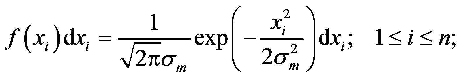
, . The special case of Gaussian distribution, which well holds for independent measures, reads:
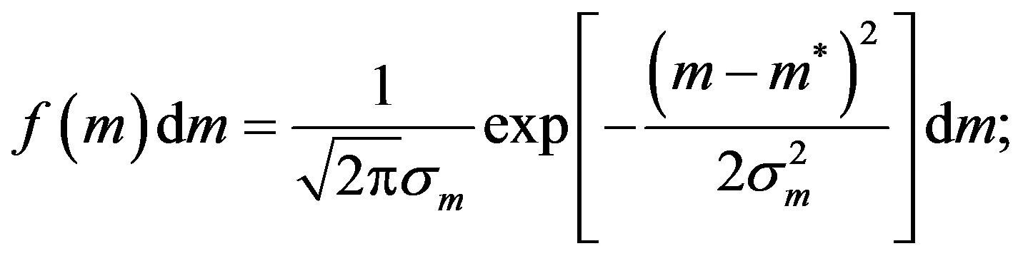 (1)
(1)
where  is a generic measure and
 ,
,  ,
,  , are the expected value, the variance, the rms error, respectively, of the distribution.
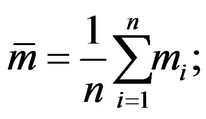
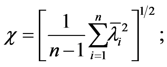
Expected value and rms error estimators are known to be the arithmetic mean,  , and the standard deviation,
  , respectively, which read:
 (2)
(2)
 (3)
(3)
 (4)
(4)
where  is the deviation from the arithmetic mean. It is worth emphasizing the bar over
  means the deviation is from the arithmetic mean:
  in itself is not an arithmetic mean. In addition, the following relations hold:
 (5)
(5)
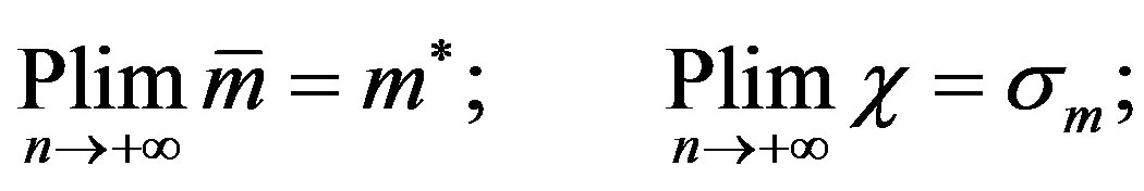
where  has to be intended in statistical sense, according to Bernoulli’s theorem (e.g., [6], Chap. 3,
  3; [7], Chap. 2,
  13; [8], Chap. 2).
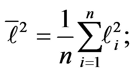
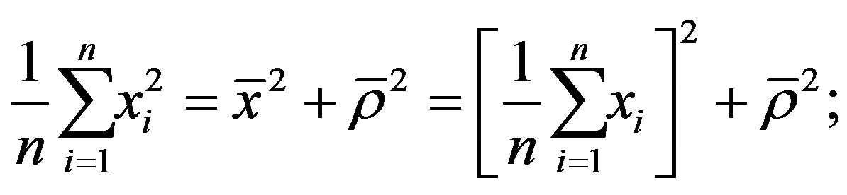
The arithmetic mean rms error and standard deviation read:
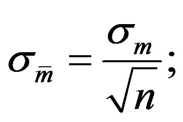 (6)
(6)
 (7)
(7)
where the bar over  means the standard deviation is related to the arithmetic mean:
  in itself is not an arithmetic mean.
The substitution of Equation (2) into (4) yields the explicit expression of the deviation in terms of the measures,  , as:
, as:
 (8)
(8)
where  is the Kronecker symbol.
Using a theorem of statistics (e.g., [7], Chap. 8; [8], Chap. 2), the deviation distribution reads:
 (9)
(9)
 (10)
(10)
by use of Equation (6).
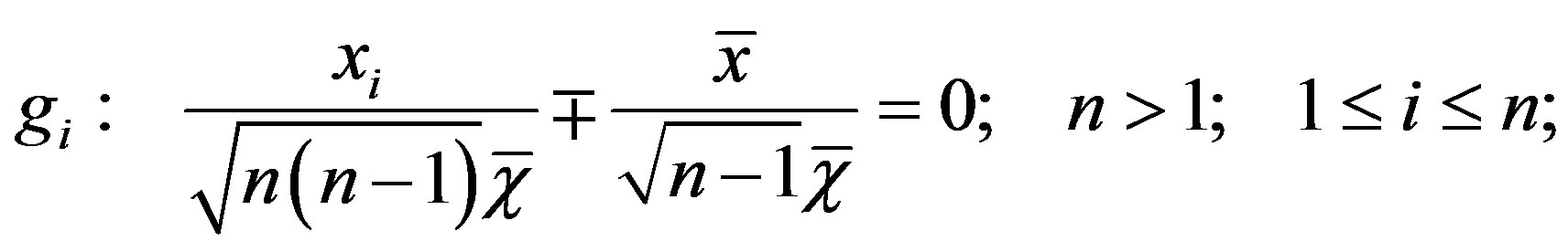
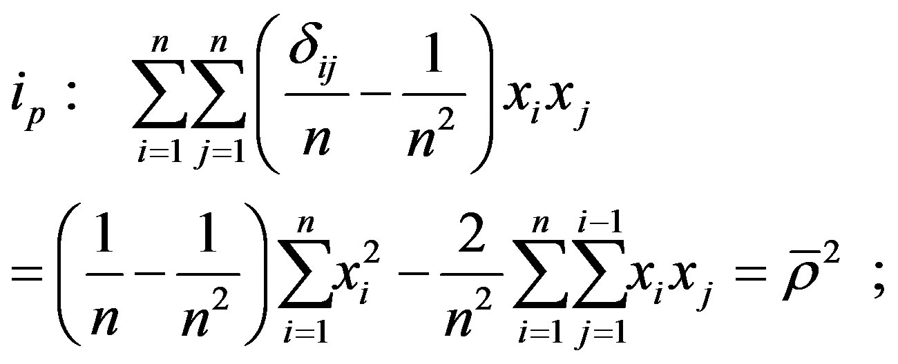
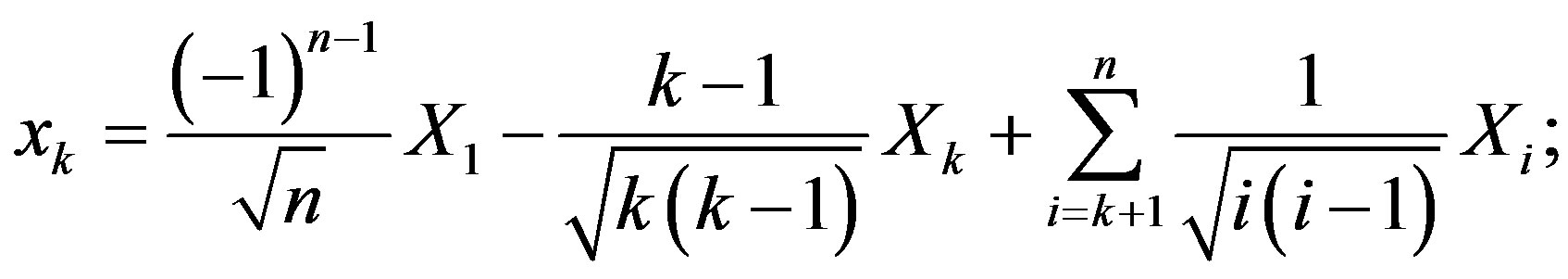
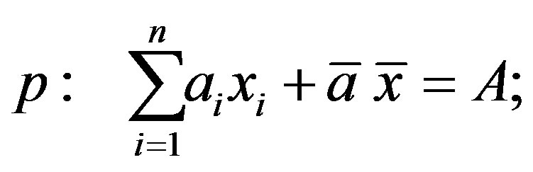
The substitution of Equation (3) into (7) yields the explicit expression of the arithmetic mean standard deviation in terms of the deviations,  , as:
, as:
 (11)
(11)
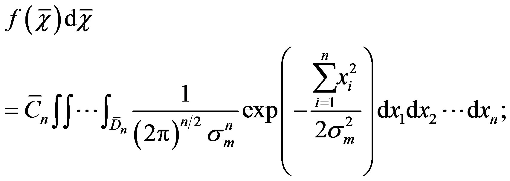
and the arithmetic mean standard deviation distribution reads:
 (12)
(12)
where the random variables,  , are no longer independent via Equation (4),
  is a normalization constant and the integration domain,
  , is made of the whole amount of n-tuples,
  which, via Equations (4), (11), define an interval, centered on
 , of infinitesimal amplitude equal to
 .
.
An explicit expression of the distribution, defined by Equation (12), is difficult to be found for two orders of reasons. First, as already mentioned, the deviations,  , are dependent random variables owing to Equation (4). Second, even
  deviations could not be considered as independent, contrary to what might be suggested by an algebraic interpretation of Equation (4). Conversely, any deviation is a function of the measures,
  , as shown by Equation (8). Accordingly, the arithmetic mean standard deviation,
  , has to be expressed in terms of independent random variables.
Aiming to calculate the multiple integral on the right-hand side of Equation (12), three steps shall be performed as outlined below.
1) Express the arithmetic mean standard deviation,  , as a function of the errors,
  , and outline the geometrical framework.
2) Express the arithmetic mean standard deviation distribution,  , as a function of the errors,
  , and outline the geometrical framework.
3) Express the arithmetic mean standard deviation distribution,  , as a function of the standard deviation,
  , the arithmetic mean rms error,
  , and outline the geometrical framework.
In dealing with the geometrical framework, for sake of simplicity, the formalism has to be specified in the following way. Hyperspaces with  dimensions, hyperplanes with
  dimensions, hyperlines with
  dimensions, hereafter shall be quoted as
  -spaces,
  -planes,
  -lines, respectively. Hypervolumes with
  dimensions, hypersurfaces with
  dimensions, hyperlengths with
  dimensions, hereafter shall be quoted as
  -volumes,
  -surfaces,
  -lengths, respectively. When the denomination of a solid is preserved, it shall be intended the symmetry is also preserved. For instance, a
  -cylinder is intended as exhibiting a single symmetry axis similarly to an ordinary cylinder.
The extension of usual formulation of analytic geometry to  -spaces, which shall be needed in the following, is outlined in Appendix.
3. Expression of  in Terms of
  and Related Geometrical Framework
The generic deviation,  , in terms of the errors,
  , can be expressed as:
 (13)
(13)
 (14)
(14)
 (15)
(15)
according to the general definition of error. It is apparent the error of the arithmetic mean equals the arithmetic mean of the errors. The substitution of Equation (15) into (13) yields:
 (16)
(16)
which shows the deviation of a measure from the arithmetic mean of the measures equals the deviation of the related error from the arithmetic mean of the errors. The right-hand side relation appearing in Equation (16) represents a n-plane passing through the origin within a  -space described by the reference frame,
  .
.
The substitution of Equation (16) into (11) after some algebra yields:
 (17)
(17)
which represents a one-sheet n-hyperboloid where the symmetry axis coincides with the coordinate axis,  , the equatorial semiaxis reads:
 (18)
(18)
and the equator is the intersection between the nhyperboloid and the principal n-plane, .
.
The asymptotes of the n-hyperboloid are generatrixes of a  -cone where the symmetry axis coincides with the coordinate axis,
  , the vertex coincides with the origin, O, and the lateral n-surface reads:
 (19)
(19)
which may be considered as the equation of the  -cone.
The generatrixes lying on the principal plane,  , are expressed as:
 (20)
(20)
which can be extended to a generic direction,  , by replacing
  with
with
 .
.
Using general formulation of analytic geometry extended to  -spaces, Equations (73) and (76), it can be seen the angle,
  , formed by the coordinate axis,
  , and the n-plane, expressed by Equation (16), equals the angle,
  , formed by the coordinate axis,
  , and the generatrixes of the
  -cone, expressed by Equation (20). Accordingly, the n-plane, expressed by Equation (16), is tangent to the
  -cone, expressed by Equation (19), along a generatrix,
  , which can be determined via the condition that the generic generatrix,
  , lies on the n-plane, expressed by Equation (16).
Keeping in mind the  -cone has vertex on the origin and symmetry axis coinciding with the coordinate axis,
  , the equation of the generic generatrix reads:
 (21)
(21)
which implies . Accordingly, Equation (19) reduces to:
 (22)
(22)
that is equivalent to:
 (23)
(23)
where, in the case under discussion of generatrixes, the square coefficient,  , equals the arithmetic mean of the square coefficients,
 . Finally, the substitution of Equation (23) into (21) yields:
 (24)
(24)
and the generatrix of interest,  , can be determined via the condition of parallelism between
  and the n-plane, expressed by Equation (16).
Owing to Equation (79), the result is:
 (25)
(25)
where, in the case under discussion of the generatrix,  , the coefficient,
  , equals the arithmetic mean of the coefficients,
 . The further condition, expressed by Equation (23), necessarily implies
  , as
, as  is needed to define a straight line in the
  -space under the validity of Equations (23) and (25).
Accordingly, the generatrix of the  -cone, defined by Equation (19), where the n-plane, defined by Equation (16), is tangent, can be expressed as:
 (26)
(26)
which is the  -sector1 of the first and 2n+1th 2n+1-ant2 of the reference frame,
 .
.
Let  be the projection of
  on the principal n-plane,
 . An explicit expression can be obtained erasing the additional coordinate,
  , from the definition of
 , Equation (26). The result is:
 (27)
(27)
which is the n-sector of the first and  th
th  -ant of the reference frame,
 .
.
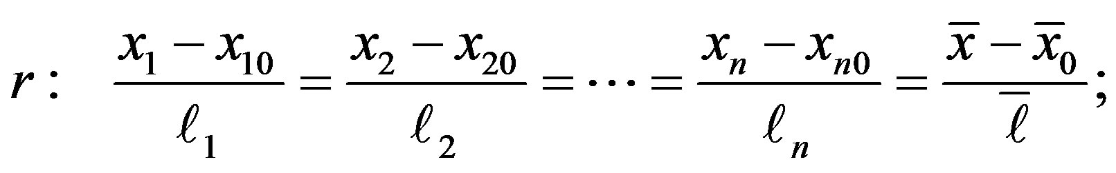
Let  be the straight
  -line, intersection between the n-plane,
  , defined by Equation (16), and the principal n-plane,
 . The expression of
  can be obtained by erasing the additional coordinate,
  , from Equation (16). The result is:
 (28)
(28)
where  passes through the origin, as expected.
Let ,
,  , be the angle formed by the straight line,
  , and the straight
  -line,
 . The particularization of Equation (73) to the case under discussion (
 ) yields:
 (29)
(29)
which implies  is normal to
 .
.
In summary, the arithmetic mean standard deviation,  , can be expressed as a function of the errors,
  , and their arithmetic mean,
  , via Equation (17), which represents a one-sheet n-hyperboloid where the symmetry axis coincides with the coordinate axis,
  , and the asymptotes are the generatrixes of a
  - cone, expressed by Equation (19), with vertex on the origin of the reference frame,
 . The condition that the sum of deviations is null, Equation (16), defines a n-plane,
  , passing through the origin, which is tangent to the above mentioned
  -cone at the generatrix,
  , coinciding with the
  -sector of the first and 2n+1th 2n+1-ant, according to Equation (26). The straight
  -line, intersection between the n-plane,
  , and the principal n-plane,
  , is normal to the projection of the generatrix,
  , on the principal n-plane,
  , according to Equation (29).
4. Expression of  in Terms of
  , and Related Geometrical Framework
According to the above results, 1) the points,  , related to a fixed value of the arithmetic mean standard deviation,
  , lie on a one-sheet
  -hyperboloid, defined by Equation (17), and 2) the points,
  , for which the sum of deviations from the arithmetic mean is null, lie on a n-plane, defined by Equation (16). The combination of Equations (15)-(17), yields:
 (30)
(30)
where the equatorial semiaxis of the  -hyperboloid,
  , is defined by Equation (18).
In terms of the errors,  , Equation (30) represents the intersection between the above mentioned
  -hyperboloid and n-plane, projected on the principal plane,
  , as:
, as:
 (31)
(31)
where, with regard to the middle side, the single sum is made of  square terms and the double sum of
  mixed products. The
  -surface,
  , is the domain of the distribution,
  , depending on the arithmetic mean standard deviation,
  , via the errors,
 . The related expression, Equation (31), is a
  -quadric where the coefficients of the firstdegree terms are null and the symmetry axis coincides with the n-sector,
  , defined by Equation (27).
The canonical form of the above mentioned  - quadric can be attained changing the reference frame from
  to
to  via rigid rotation around the origin, where the resulting coordinate axes,
  , coincide with the principal axes of the n-volume bounded by the
  -quadric and, without loss of generality,
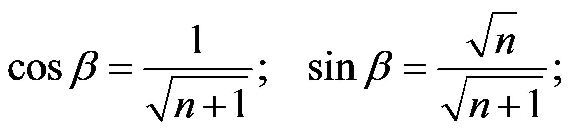
  may be chosen as symmetry axis. To this aim, the direction cosines must be determined where, in general,
  is the cosine of the angle formed by the resulting coordinate axis,
  , and the starting coordinate axis,
  ,
,  ,
, .
.
The extension of standard relations involving direction cosines to n-spaces yields:
 (32)
(32)
 (33)
(33)
and the condition of parallelism and orthogonality between coordinate axes read:
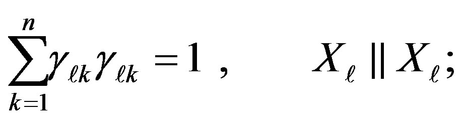 (34)
(34)
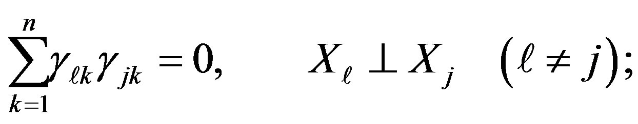 (35)
(35)
with regard to the starting reference frame,  , and:
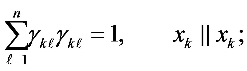 (36)
(36)
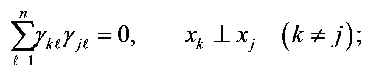 (37)
(37)
with regard to the resulting reference frame,  .
.
The validity of Equations (34)-(37) implies the orthogonality of the Jacobian determinant:
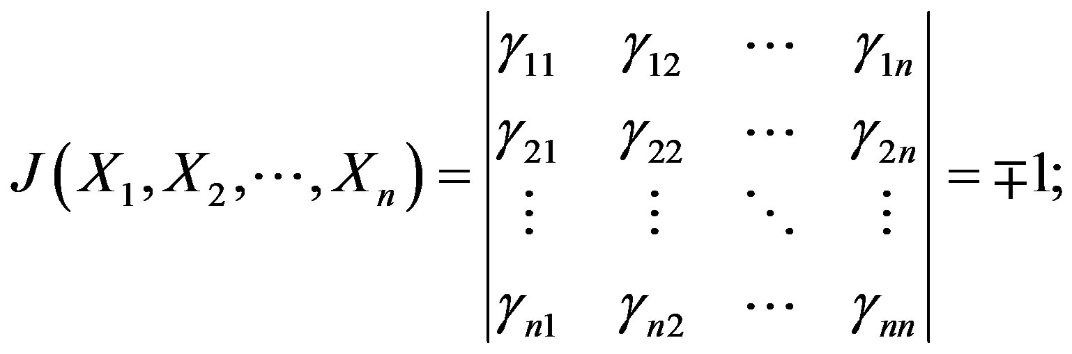 (38)
(38)
where the positive value relates to a rigid rotation of the starting reference frame around the coordinate axis,  , i.e. within the principal n-plane,
  , while the negative value relates, in addition, to an odd number of rigid rotations by an angle,
  , each around a different coordinate axis,
  ,
,  , i.e. outside the principal n-plane,
 .
.
Owing to Equation (27), the symmetry axis,  , coincides with the n-sector of the first and 2nth 2n-ant of the starting reference frame. Accordingly, related direction cosines are equal and can be inferred from Equation (76) particularizing the straight lines,
  and
and , to the n-sector,
  , and the coordinate axis,
  ,
,  respectively, which implies
 ;
;
 ; and Equation (76) reduces to:
 (39)
(39)
which, in turn, implies:
 (40)
(40)
with regard to the direction cosines involving the coordinate axis, . The remaining coordinate axes,
  , can be arbitrarily selected, according to Equations (34) and (35), in that they are related to the
  principal axes of the
  -circle, centered on the origin and normal to the coordinate axis,
 . For this reason, the starting and the resulting reference frame are not needed to be congruent provided the Jacobian determinant is orthogonal according to Equation (38).
Following the above mentioned procedure with regard to the resulting reference frame,  , Equation (32) takes the explicit expression:
 (41)
(41)
and the direction cosine,  , by definition, can be inferred from Equation (41) replacing
  by
by  and
and  by the Kronecker symbol,
 . The result is:
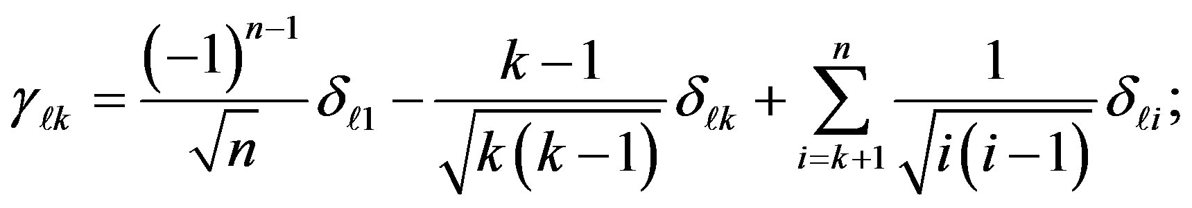 (42)
(42)
where the power,  , ensures congruence (not needed, as mentioned above) between the starting and the resulting reference frame.
The substitution of Equations (40) and (42) into (38), after some determinant algebra, yields the explicit expression of the Jacobian determinant, as:
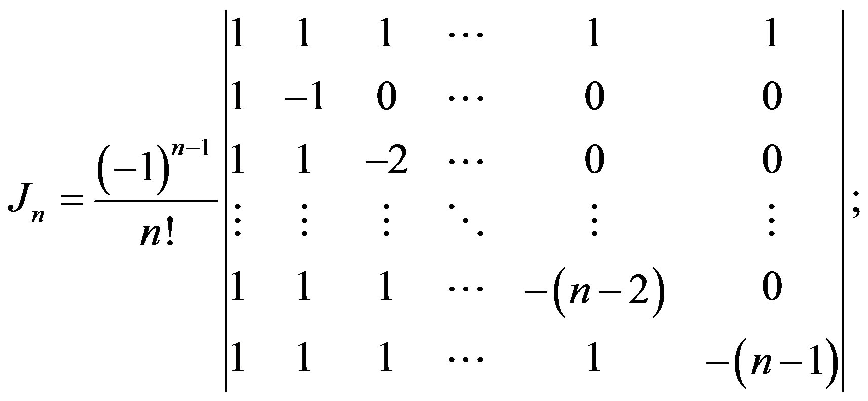 (43)
(43)
which, after additional determinant algebra, takes the expression:
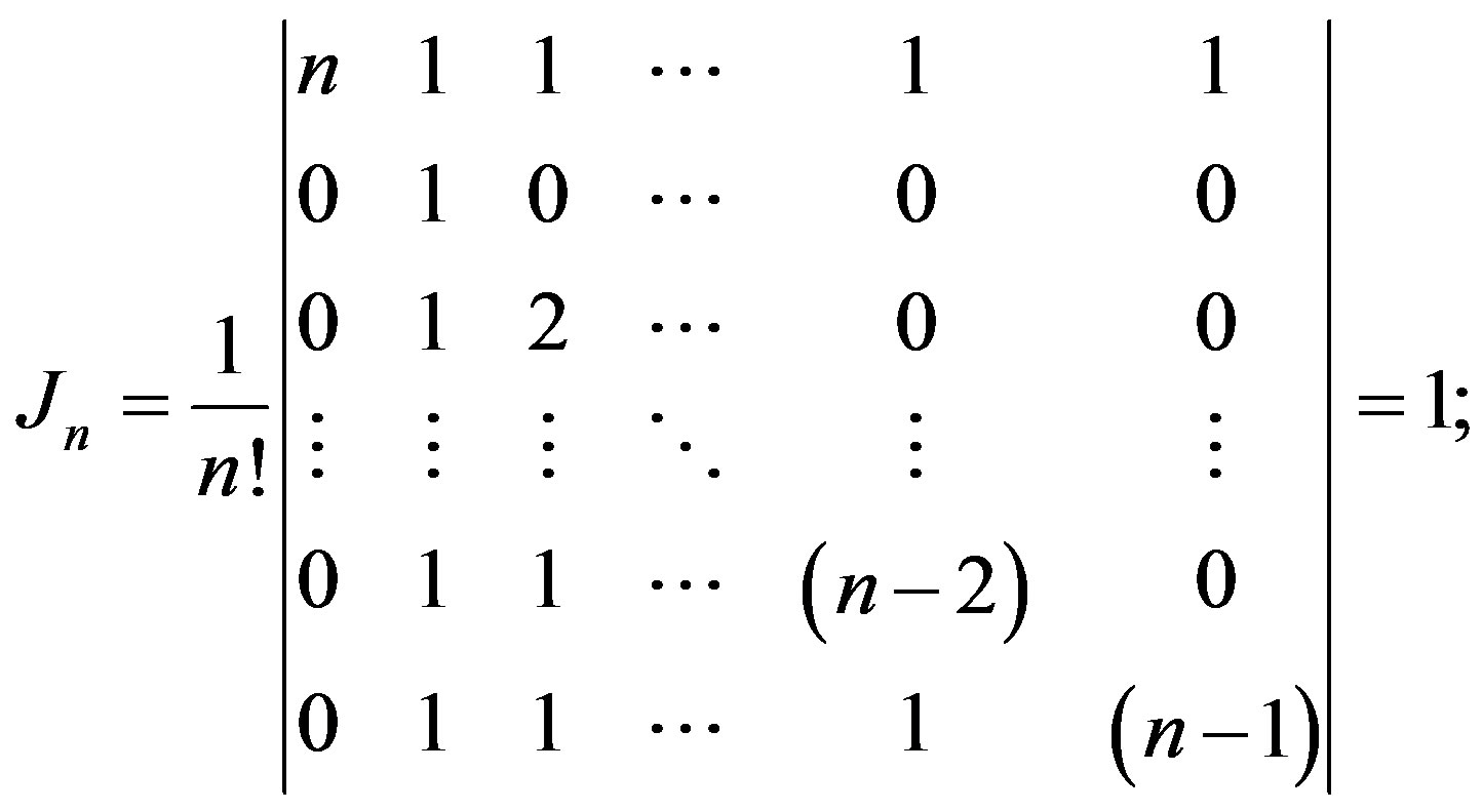 (44)
(44)
in agreement with Equation (38).
Particularizing Equation (41) to , respectively, and performing the sum on the left and righthand side, after some algebra yields:
 (45)
(45)
on the other hand, the invariance of the norm by changing the reference frame implies the following:
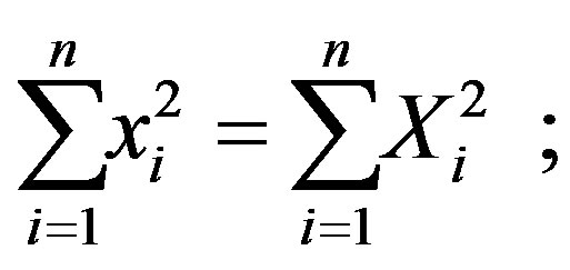 (46)
(46)
and the substitution of Equations (45) and (46) into (30) yields:
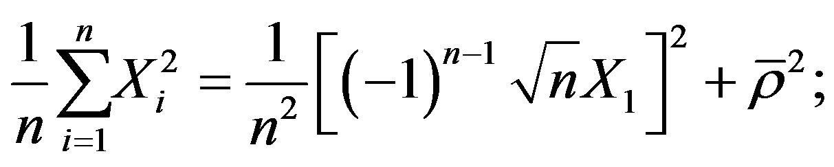 (47)
(47)
which, using Equation (18), after some algebra produces:
 (48)
(48)
that is the locus of  -circles normal to the coordinate axis,
  , centered therein, where the radius is:
 (49)
(49)
in other terms, Equation (48) defines a n-cylinder where the symmetry axis coincides with the coordinate axis,  , and the radius equals
 .
.
In summary, the arithmetic mean standard deviation distribution can be expressed as a function of the errors,  , as:
, as:
 (50)
(50)
where  is a normalization constant,
  the integration domain, expressed by Equation (31) which, turned into canonical form, Equation (48), represents a n-cylinder of infinite height, symmetry axis coinciding with the coordinate axis,
  , and radius defined by Equation (49).
Finally,  ,
,  , are error distributions expressed via Equation (1) as:
 (51)
(51)
where  is the related rms error.
5. Expression of  in Terms of
 ,
,  , and Related Geometrical Framework
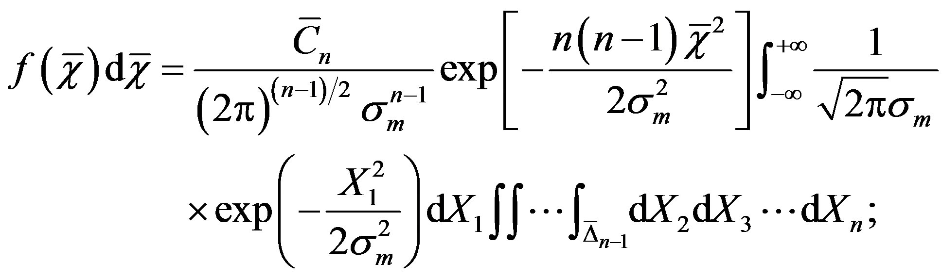
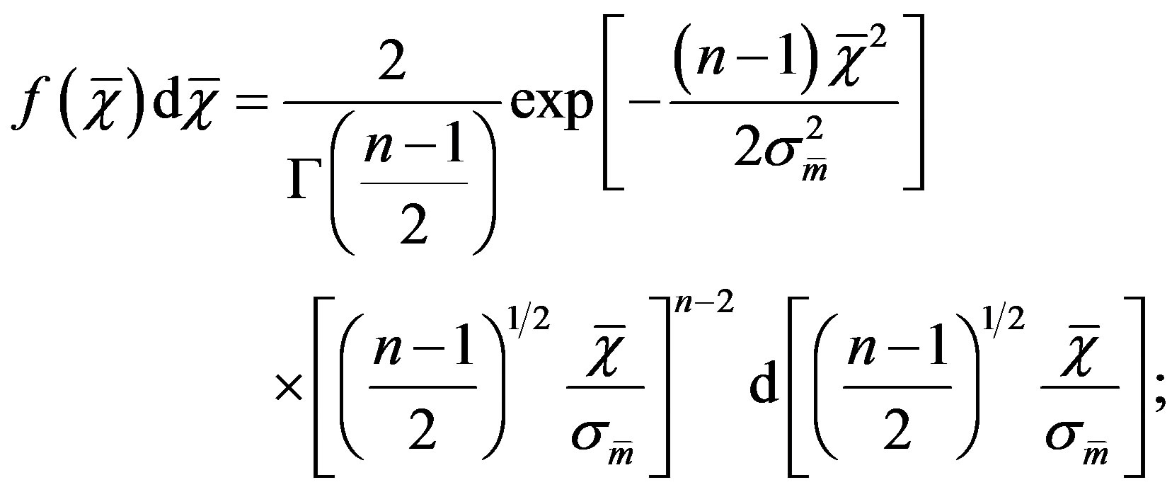
The substitution of Equation (51) into (50) after little algebra yields:
 (52)
(52)
the special case,  , is shown in Figure 1.
With regard to the resulting reference frame,  , after a change of variables (e.g., [9], Chap. III,
  4.10; [8], Chap. 4) by use of Equation (46), Equation (52) translates into:
 (53)
(53)
where the integration domain,  , is an infinitely thin n-cylindrical corona with symmetry axis,
  , and radius defined by Equation (49).
Then the substitution of Equation (38) and (48) into (53) yields:
 (54)
(54)
the special case,  , is shown in Figure 2.
With regard to the principal  -plane,
  , the
, the  -surface of the
  - circle of radius,
  , is (e.g., [10], Mathematical Appendix):
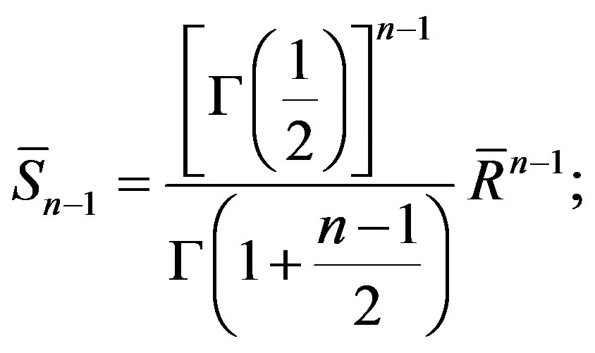 (55)
(55)
where  is the Euler Gamma function, which satisfies the following relations (e.g., [11], Chap. 39,
  39.6):
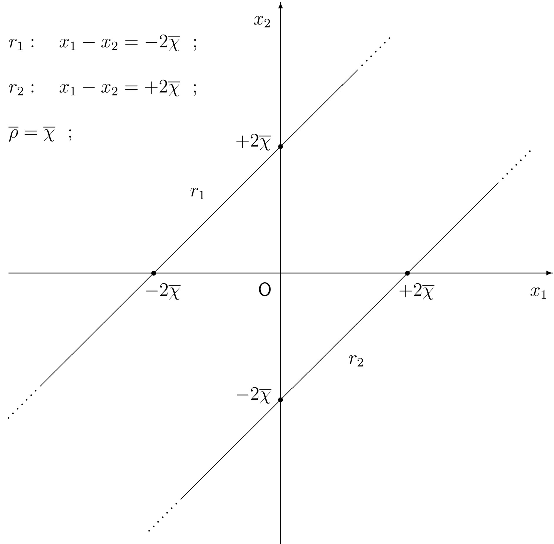
Figure 1. The integration domain,  , with regard to the reference frame,
  , in the special case,
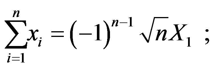
 . The straight lines,
  ,
,  , are the axes of infinitely thin bands, whose bounderies are defined by the straight lines,
 ;
; . The integration domain,
  , is defined by the above mentioned bands.

Figure 2. The integration domain,  , with regard to the reference frame,
  , in the special case,
 . The straight lines,
  ,
,  , are the axes of infinitely thin bands, whose boundaries are defined by the straight lines,
 ;
; ; according to Equation (48). The integration domain,
  , is defined by the above mentioned bands.
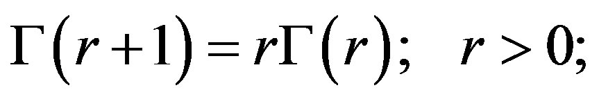 (56a)
(56a)
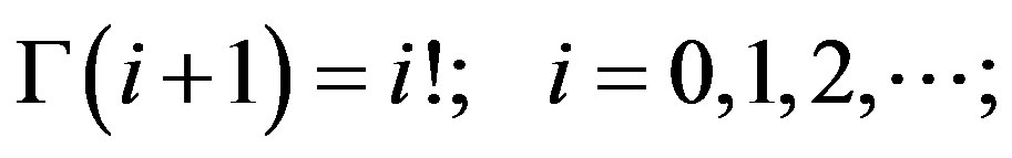 (56b)
(56b)
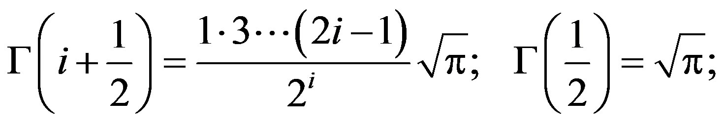 (56c)
(56c)
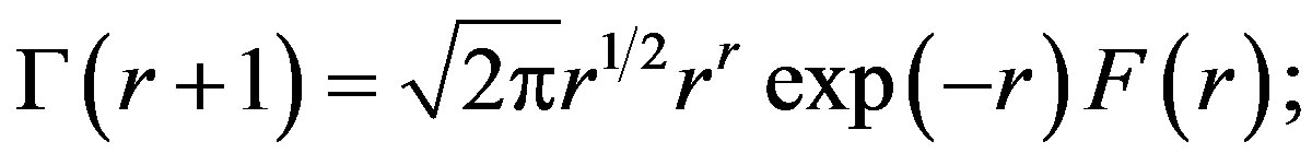 (56d)
(56d)
 (56e)
(56e)
and the particularization of Equation (55) to the simplest cases,  yields:
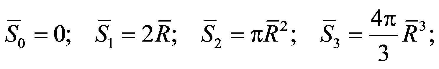 (57)
(57)
with regard to points, segments, circles, spheres, respectively.
In particular,  implies a single deviation from the mean,
  according to Equation (4), then
  via Equations (11) and (49). Accordingly, the 0-circle coincides with the origin of the reference frame,
  , the 0-surface of which is clearly null. For this reason, the undetermined expression,
  as
as , appearing in Equation (55), may safely be put equal to 0, hence
 , in agreement with Equation (57). On the other hand, Equations (17), (19), (20), lose their validity for
 .
.
The  -surface of an infinitely thin
  - circular corona can be determined by differentiating both sides of Equation (55). The result is:
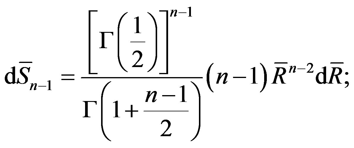 (58)
(58)
which is independent of the reference frame.
In summary, the arithmetic mean standard deviation distribution,  , may be expressed as a multiple integral where the integration domain,
  , is an infinitely thin n-cylindrical corona where the symmetry axis coincides with the coordinate axis,
  , and the radius is defined by Equation (49). The result, expressed by Equation (54), after some algebra takes the form:
 (59)
(59)
where the integration domain of the ordinary and the multiple integral are the symmetry axis and the  - circular section of the n-cyclindrical corona, respectively, hence
 .
.
6. The Solution
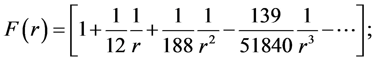
The substitution of Equations (18), (58), into (59), after long but stimulating algebra yields:
 (60)
(60)
where  is the arithmetic mean rms error, Equation (6), and due account has been paid to Equations (56a), (56c), together with the normalization condition:
 (61)
(61)
which, after integration as outlined above via Equation (59), is equivalent to:
 (62)
(62)
according to Equation (60) that, in addition, can be related to a chi square distribution with  degrees of freedom.
The expected values,  ,
,  , can be determined starting from the general definition:
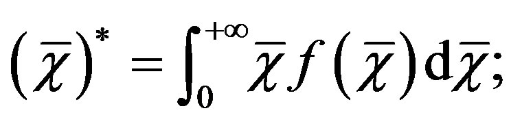 (63)
(63)
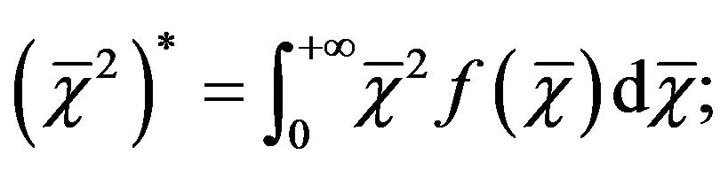 (64)
(64)
by substitution of Equation (60) into (63) and (64). After long but stimulating algebra, the integration yields:
 (65)
(65)
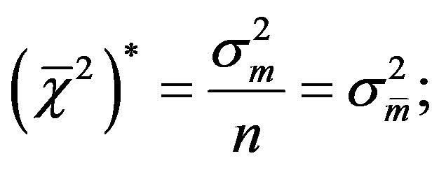 (66)
(66)
and the rms error of the arithmetic mean standard deviation distribution, 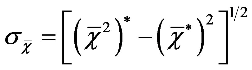 , after some algebra reads:
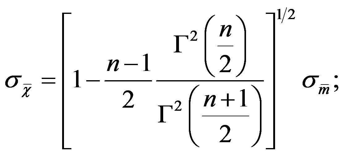 (67)
(67)
by use of Equations (65) and (66).
The validity of the asymptotic expression (e.g., [8]):
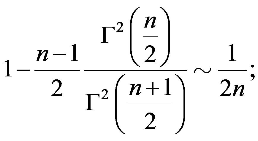 (68)
(68)
together with the inequalities:
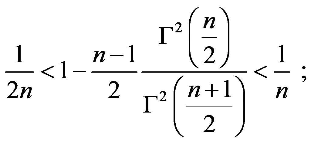 (69)
(69)
imply for Equation (67) the asymptotic expression (e.g., [8]):
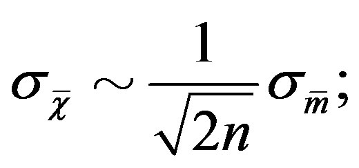 (70)
(70)
where the ratio,  , is understimated according to Equations (67) and (69).
In summary, the arithmetic mean standard deviation distribution is explicitly expressed by Equation (60) and related expectation values,  ,
,  , and rms error,
 , are expressed by Equations (65)-(67), respectively. Finally, an asymptotic expression of
  is shown by Equation (70), where the value is understimated.
7. Conclusions
The arithmetic mean standard deviation distribution and related parameters have been determined following a procedure where the geometrical framework is clearly shown using typical formulation generalized to n-spaces. The integration has been performed after a change of reference frame, where the integration domain turns out to be an infinitely thin n-cylindrical corona that is symmetric with respect to a coordinate axis.
Although alternative approaches grounded on mathematical analysis and statistics could appear shorter and less coumbersome, still the geometrical features are lost. A geometrical interpretation is essential in modern physical, cosmological and elementary particle theories, such as general relativity, superstring theory and supersymmetric theory. In this view, an investigation of the geometrical framework related to any field e.g., mechanics, statistics, crystallography, music, could be of some utility.
8. Acknowledgements
A more extended version of the current attempt appears in the last edition (in Italian, unpublished) of the quoted text [8] by the author.
REFERENCES
- C. W. Misner, J. A. Wheeler and K. S. Thorne, “Gravitation,” W.H. Freeman & Company, 1973.
- B. Greene, “The Elegant Universe: Superstrings, Hidden Dimensions, and the Quest for the Ultimate Theory,” W.W. Norton, 1999.
- J. Douthett and R. Krantz, “Energy Extremes and Spin Configurations for the One-Dimensional Antiferromagnetic Ising Model with Arbitrary-Range Interactions,” Journal of Mathematical Physics, Vol. 37, No. 7, 1996, pp. 3334-3353. http://dx.doi.org/10.1063/1.531568
- A. M. Kosevich, “The Crystal Lattice: Phonons, Solitons, Dislocations, Superlattices,” WILEY-VCH Verlag GmbH & Co. KGaA, Weinheim, 2005.
- C. Callender, I. Quinn and D. Tymoczko, “Generalized Voice-Leading Spaces,” Science, Vol. 320, No. 5874, 2008, pp. 346-348. http://dx.doi.org/10.1126/science.1153021
- A. Papoulis, “Probabilities, Random Variables, and Stochastic Processes,” McGraw-Hill, New York, 1965.
- B. Gnedenko, “The Theory of Probability,” Mir, Moscow, 1978.
- R. Caimmi, “Il Problema della Misura,” Diade, Nuova Vita, Padova, 2000.
- V. Smirnov, “Cours de Mathèmatiques Supèrieures,” Tome II, Mir, Moscow, 1970.
- B. B. Mandelbrot, “Les Objects Fractals: Forme, Hazard et Dimensions,” 2nd Edition, Flammarion, Paris, 1986.
- M. R. Spiegel, “Mathematical Handbook of Formulas and Tables,” Schaum’s Outline Series, McGraw-Hill, New York, 1969.
Appendix
Analytic Geometry Formulation Extended to  -Spaces
Analytic geometry formulation extended to  - spaces, used throughout the text, is outlined below. It shall be intended, but not explicitly mentioned where unnecessary, that the reference frame is
 .
.
Let  and
and  be a generic straight line and n-plane, respectively, defined as:
 (71)
(71)
 (72)
(72)
where  is a fixed point belonging to
  and
and ,
, ;
; ,
,  , A; are specified coefficients.
Let ,
,  , be the angle formed by the straight line and the n-plane. Related trigonometric functions can be inferred from the explicit expression of the sine, as:
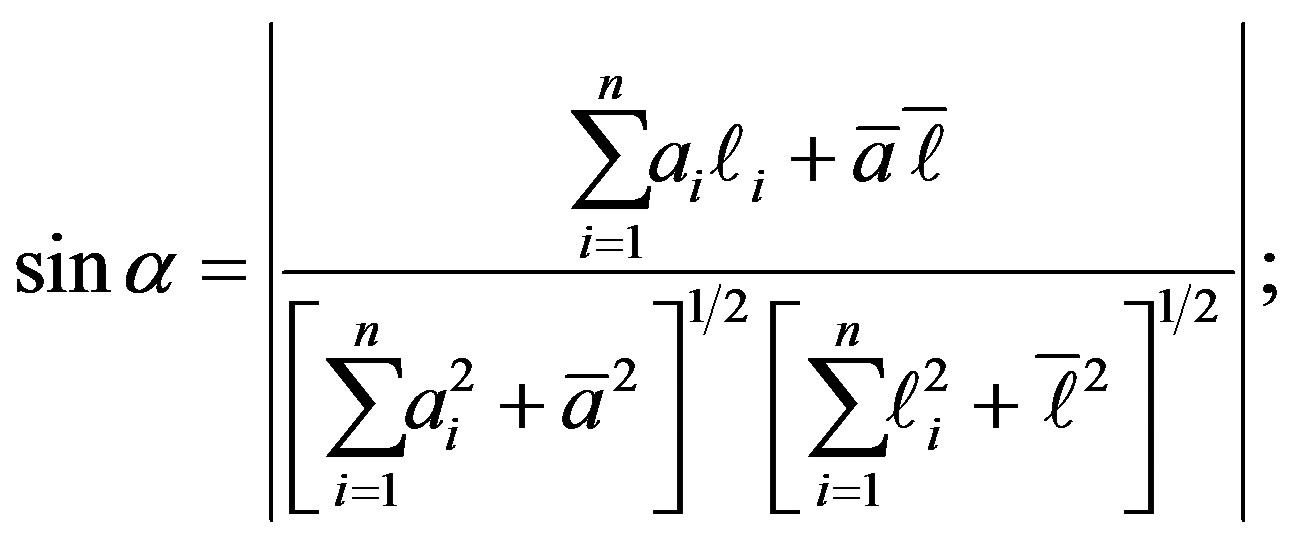 (73)
(73)
which, in the case of interest 
 , reduces to:
 (74)
(74)
where  coincides with the coordinate axis,
  , and
, and  passes through the origin.
Let  be a generic straight line, defined as:
 (75)
(75)
where  is a fixed point belonging to
  and
and , are specified coefficients.
Let ,
,  , be the angle formed by the straight lines,
  and
and . Related trigonometric functions can be inferred from the explicit expression of the cosine, as:
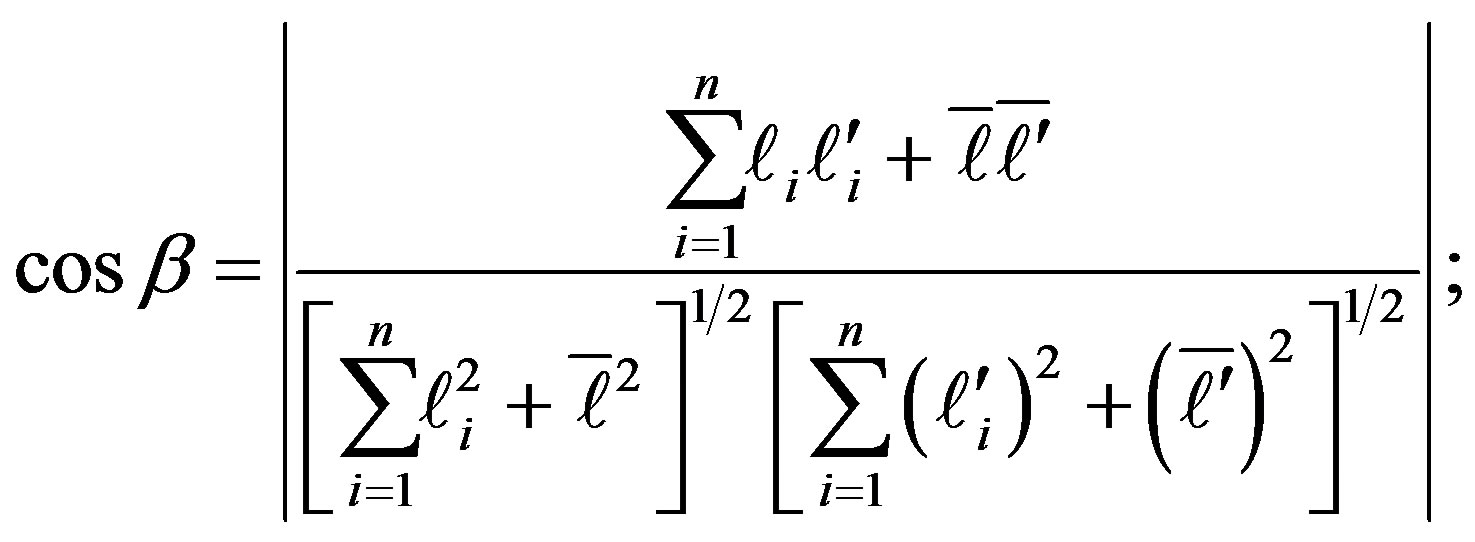 (76)
(76)
which, in the case of interest ( ,
, ;
; ;
; ;
; ,
, ;
; ), reduces to:
 (77)
(77)
where  is the generatrix, lying on the principal plane,
  , of the
  -cone, defined by Equation (19), and
  coincides with the coordinate axis,
 .
.
The condition of parallelism between the straight line,  , and the n-plane,
  , reads:
 (78)
(78)
which, in the case of interest (
 ), reduces to:
 (79)
(79)
where  is the n-plane, defined by Equation (16).
NOTES
1In particular, 2-sector reads bisector, 3-sector reads trisector, 4-sector reads quadrisector, and so on.
2In particular, 2-ant reads versant, 4-ant reads quadrant, 8-ant reads octant, and so on.