Applied Mathematics
Vol.3 No.10(2012), Article ID:23376,6 pages DOI:10.4236/am.2012.310162
Two Implicit Runge-Kutta Methods for Stochastic Differential Equation
Department of Mathematics, University of Electronic Science and Technology of China, Chengdu, China
Email: zhywang@uestc.edu.cn
Received August 20, 2012; revised September 10, 2012; accepted September 17, 2012
Keywords: Stochastic Differential Equation; Implicit Stochastic Runge-Kutta Method; Order Condition
ABSTRACT
In this paper, the Itô-Taylor expansion of stochastic differential equation is briefly introduced. The colored rooted tree theory is applied to derive strong order 1.0 implicit stochastic Runge-Kutta method (SRK). Two fully implicit schemes are presented and their stability qualities are discussed. And the numerical report illustrates the better numerical behavior.
1. Introduction
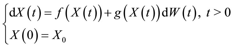
In this paper, we want to obtain numerical methods for strong solution of Stochastic Differential Equations of Itô type.
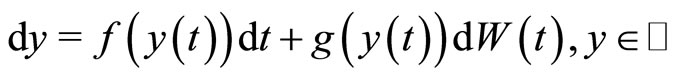 (1.1)
(1.1)
Note that f is a slowly varying continuous component function, which is called drift coefficient,  is the rapidly varying continuous function called the diffusion coefficient.
  is a wiener process.
Recently, many scholars have successfully derived some methods for SDEs for both Itô and Stratonovich forms. Burrage and Burrage [1-3] established the colored rooted tree theory and Stochastic B-series expansion. Tian and Burrage [2,4,5] derived some strong order 1.0 2-stage Stochastic Runge-Kutta methods, including semiimplicit and implicit methods. Wang P. [6] derived some strong order 1.0 3-stage semi-implicit methods. Wang ZY [7] mainly considered the strong order SRKs for the SDEs of Itô form. In his PhD thesis he offered us the Colored Rooted tree theory for Itô tpye, and constructed some 2-stage and 3-stage explicit methods. Along this line, I will construct some implicit SRKs for SDEs of Itô type. In Section 2, the colored rooted tree theory for deriving SRK for SDEs of Itô type is briefly introduced and the 2 2-stage fully implicit SRKs are obtained. In Section 3 we will discuss their stability property. And in Section 4, we will report the numerical experiments.
2. 2-Stage Implicit SRK and Order Conditions
Many scholars, including Burrage [2], offered the definition of the order of numerical methods in their thesis.
Definition 2.1. Let  be the numerical approximation to
  after N steps with constant stepsize
 ; then
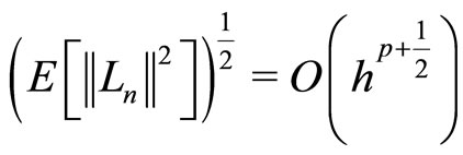
  is said to be converge strongly to
  with order
  if
if
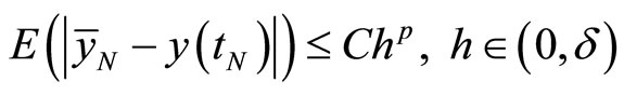 (2.1)
(2.1)
Note that  is a constant that independent of h and
 .
.
Butcher presented the Rooted Tree theory, after which this theory was extended into stochastic area. Burrage [2] presented Colored Rooted Tree theory in her PhD thesis, and Wang [7] did the research especially for Itô SDEs. Similar to the deterministic condition, the definition of the elementary differential can be associated with 


Here  stands for the trees having order 0.
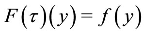
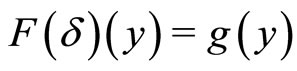
Wang [7] deduced the Itô-Taylor series for SDEs. Firstly let’s introduce two operators
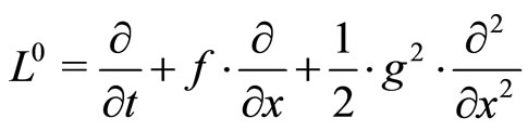
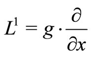
Now we introduce a very important proposition from Kloeden and Platen [8].
Proposition 2.1. if ,
,  is sufficiently derivative, and let X(t) be the solution of the equation
then
 (2.2)
(2.2)
Letting , then
And from the definition of the elementary differential we can know
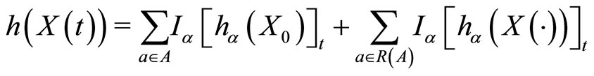
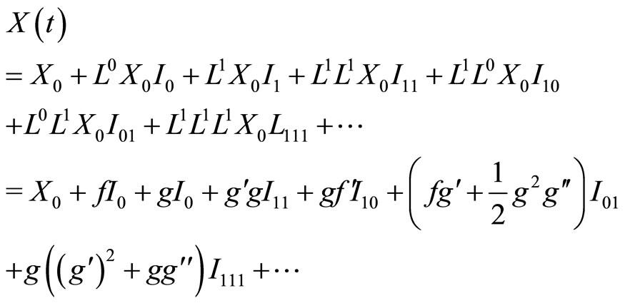
Like the conclusion of Burrage [2], the Taylor-series of the actual solution of the SDEs is
 (2.3)
(2.3)
The structure of Stratonovich-Taylor series is similar to the Itô-Taylor expansion, however, the stochastic calculations of these two types are different. Table 1 presents the trees and the corresponding elementary differentials. Especially, in order to illustrate the difference between Itô type and stratonovich type, we list all the stochastic calculations of trees having order  2.
2.
Now we show general form of Runge-Kutta methods for SDEs of Itô form. Let the stepsize of the methods is a constant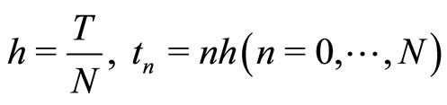 , yn is the numerical solution of
 , then
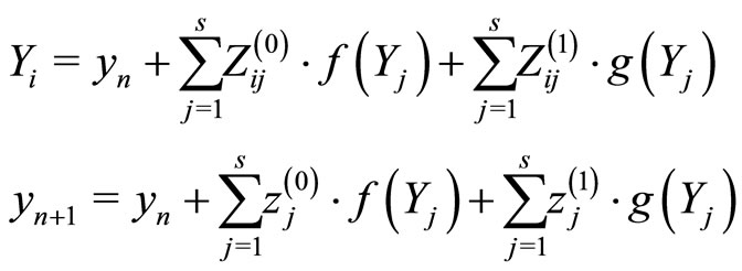 (2.4)
(2.4)
Note that
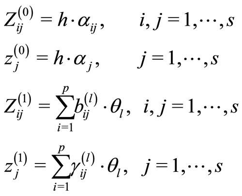
where the  is random variables.
Using the Butcher Table, SRK can be written as

Wang [7] deduced the Taylor series for the SRK of Itô form. And offered the definition of Elementary Weight, which has the same form of Burrage’s conclusion [2].
Definition 2.2.
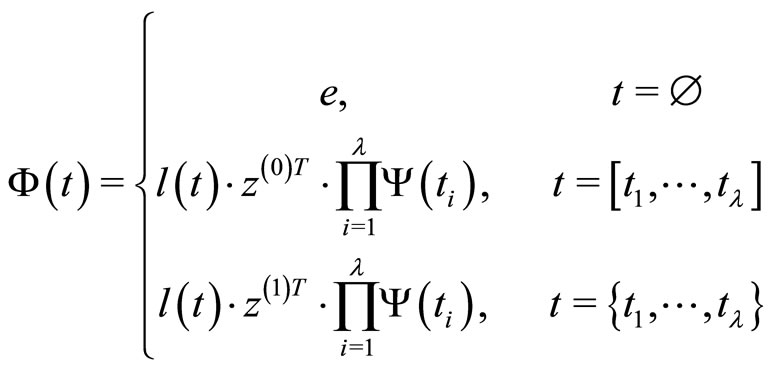
where
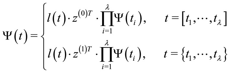
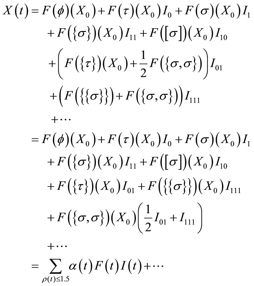
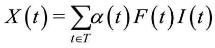
As the definition of Elementary Weight that we obtained, we can gain the stochastic Runge-Kutta series expansion
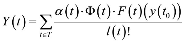 (2.5)
(2.5)
Table 2 offers the trees and their Elementary Weights.
From the Equations (2.4) and (2.5) we can obtain the truncation error at .
.

Table 1. Trees and the corresponding elementary differentials.
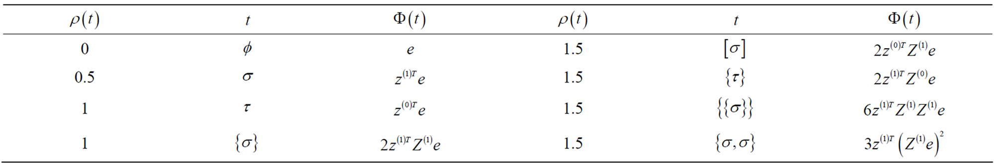
Table 2. Trees and the corresponding elementary weights.
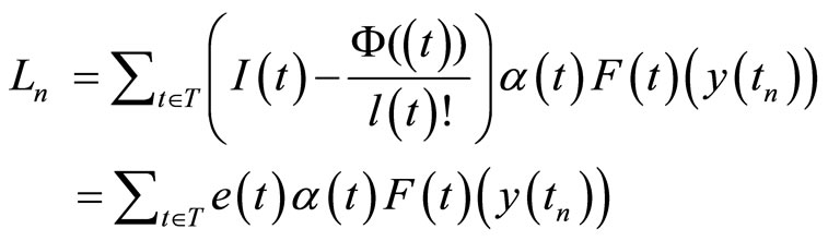
Proposition 2.2, given by Burrage and Burrage [3], gives the necessary conditions of the methods.
Proposition 2.2.  is the local truncation error of the numerical methods at
 ,
,  is the global error at
 , if f and g is sufficiently derivative, and

then
From the Proposition 2.2, the Runge-Kutta methods of the strong order 1.0 have to satisfy
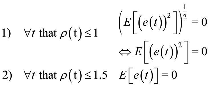 (2.6)
(2.6)
obviously,  ,
,  , thus in 2) We just need to consider the condition when
 .
.
Now we introduce the random variables  . And we note
Now let’s start to construct the methods of strong order 1.0.
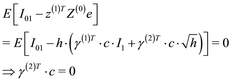
1) For tree 
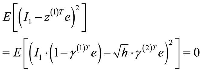
namely
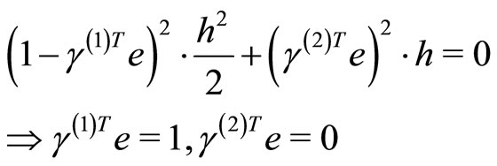
2) For tree 
3) For tree 
namely
where

and
namely
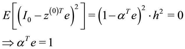
4) For tree 
5) For tree 
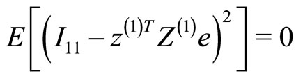
6) For tree 
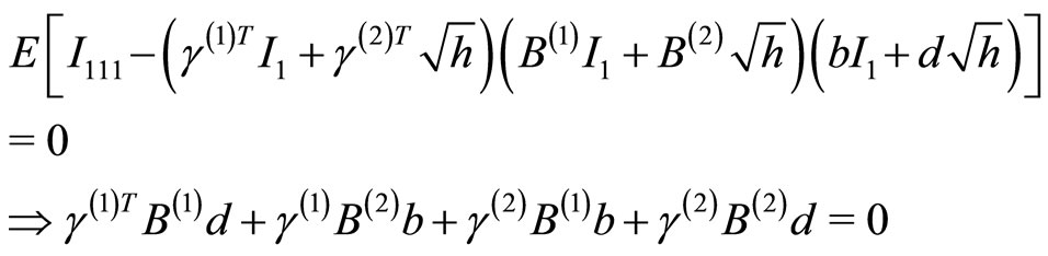
7) For tree 
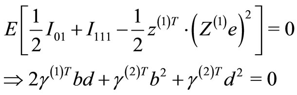
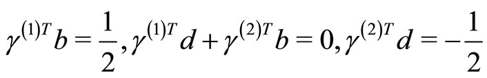
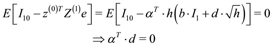
Thus, the 2-stage implicit SRKs should satisfy the system
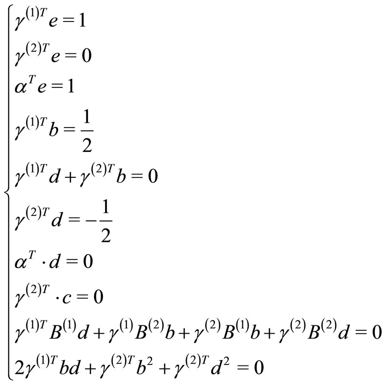 (2.7)
(2.7)
Here we gained the conditions for the methods with strong order 1.0, theoretically we can construct any-stage methods, both explicit and implicit. And now we consider the 2-stage implicit methods.

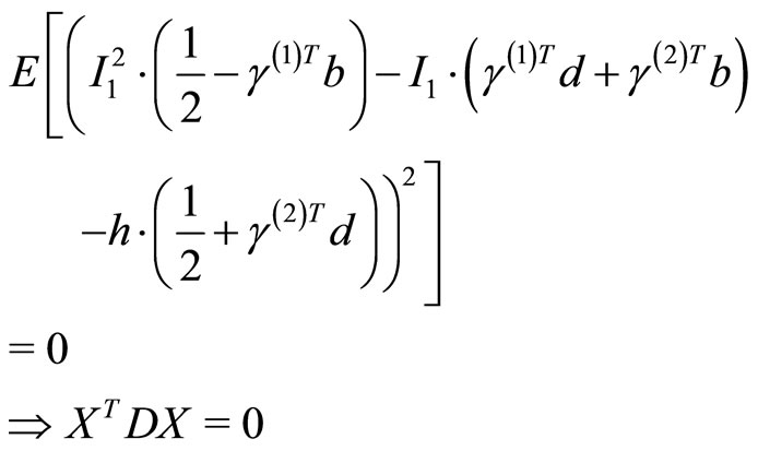
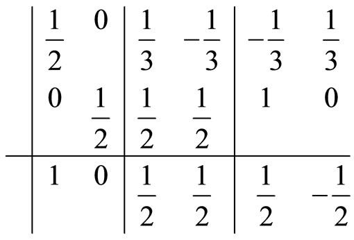
Bringing the table into the system 2.7, and letting the
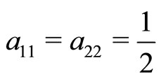 ,
,  ,
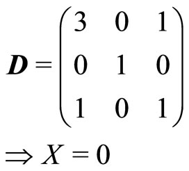
,  , we can obtain the first scheme—

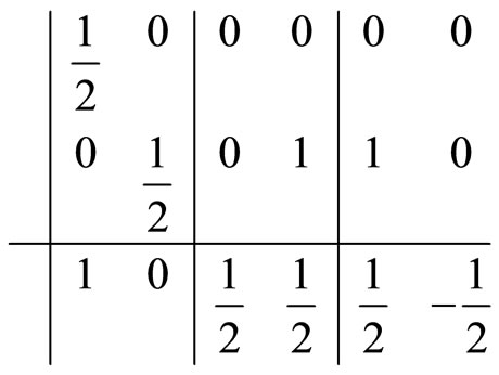
Furthermore if we continue to let 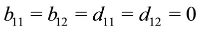 , we can obtain another scheme —
 .
.

3. Stability
Saito and Mitzui [9] introduced the definition of meansquare(MS) stability, and the scholars such as Burrage [2] and Tian [4,5] researched it and gave some improvements.
Consider the linear test equation of Itô type of SDEs.
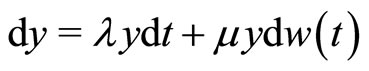 (3.1)
(3.1)
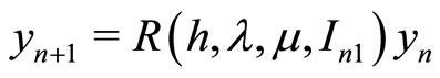
and we use one-step scheme

where h is the stepsize,  is the random variable in the numerical scheme.
Satio and Mitzui [9] introduced the definition Definition 3.1. If for ,
,
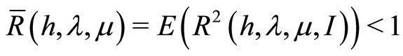
then the numerical scheme is said to be MS stable, and the 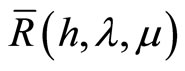 is said to be the MS-stability function.
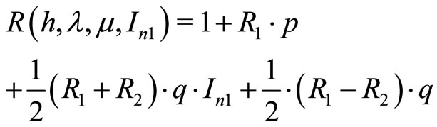
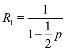
1) For , we can obtain the MS-stability function

where
Note that
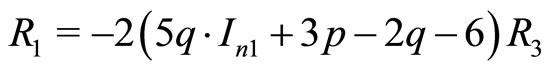
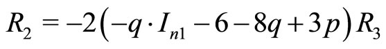
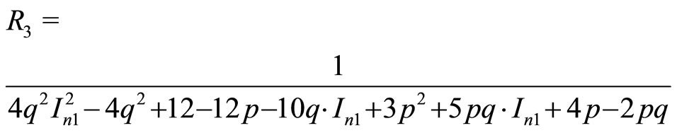
and
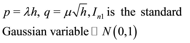
Figure 1 describes the stable region of .
.
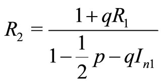
2) For the method , we obtain that
where

Note that
and
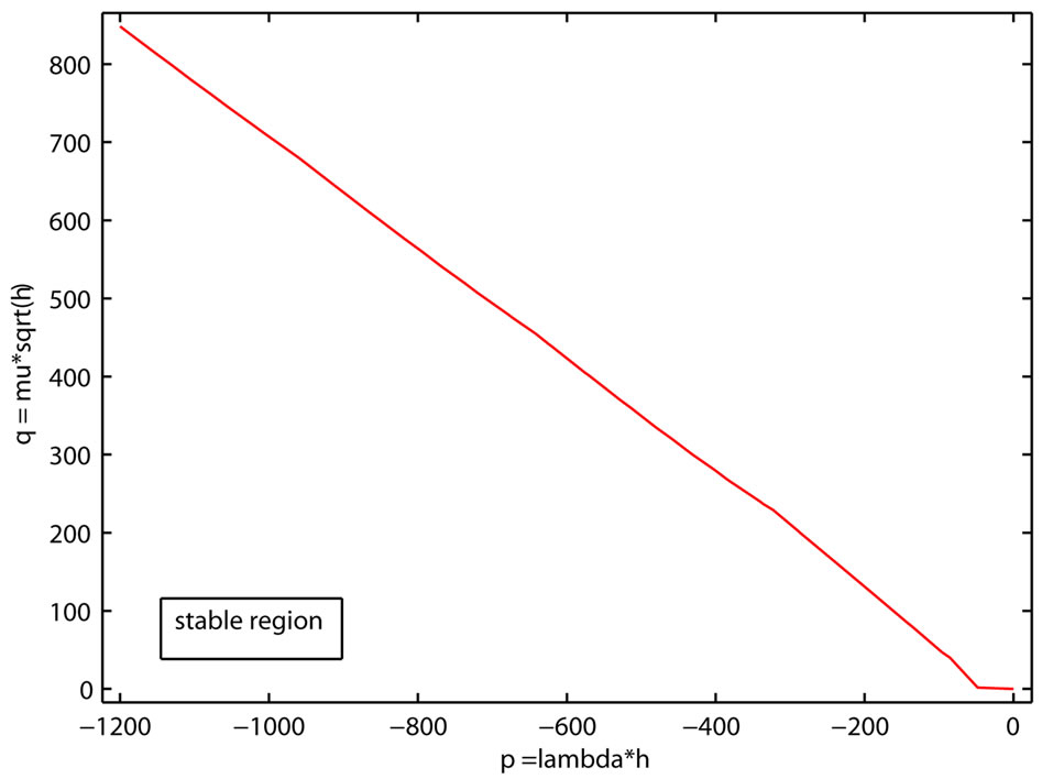
Figure 1. Stable region of Imp1.
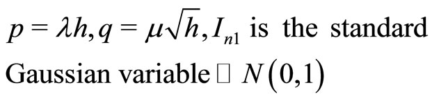
Figure 2 represents the stable region of .
.
4. Numerical Results
Now we report the numerical results of the schemes derived in this paper. At first we will use the points of numerical simulation in a single trajectory to compare the absolute error Ms of five different schemes—explicit Euler-Maruyama scheme, explicit milstein scheme, explicit two-stage scheme  which is designed by Wang [7],
  and
and —for a same non-linear system 10. After which we will simulate 100 trajectories of each scheme and then compare their absolute error Ms.
Errors for the (4.1) is given by
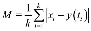
Note that  is the exact value at step point
  and
and  is the numerical simulation at that point,
  is the number of the points chosen in the trajectories. And the non-linear system (4.1) is given by
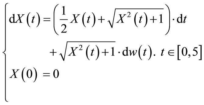 (4.1)
(4.1)
And the analytical solution of the system 10 is
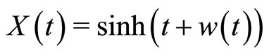 (4.2)
(4.2)
Firstly, we compare the error Ms in a single trajectory. From the Table 3, we can know that in a random trajectory(actually we choose the first one), the  is obviously better than all the other schemes, and also,
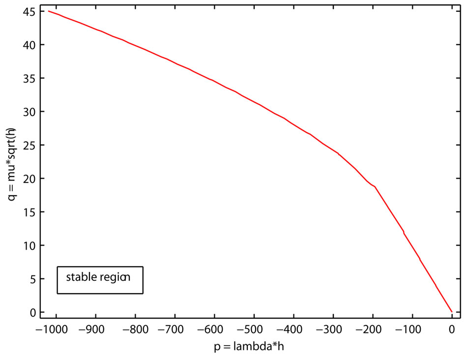
Figure 2. Stable region of Imp2.

Table 3. The absolute error Ms in a single trajectory.
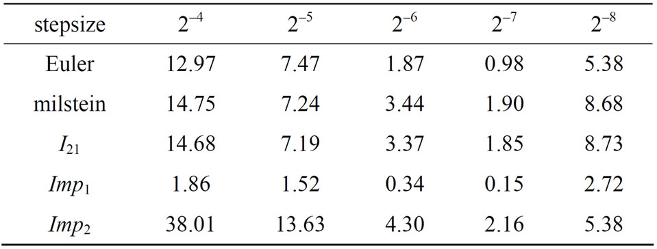
Table 4. Mean of the absolute error Ms in 100 trajectories.
 has a same accuracy with
  scheme and milstein scheme.
Now let’s contrast the absolute error Ms of 100 trajectories.
From the Table 4, we can conclude that  is obviously better than all the other schemes, especially when
 . Still,
  always has a same accuracy with
  scheme and milstein scheme. It shows that
  is better than other schemes, and
  is also a proper scheme for solving stochastic differential equations.
REFERENCES
- K. Burrage and P. M. Burrage, “High Strong Order Explicit Runge-Kutta Methods for Stochastic Ordinary Differential Equations,” Applied Numerical Mathematics, Vol. 22, 1996, pp. 81-101. doi:10.1016/S0168-9274(96)00027-X
- P. M. Burrage, “Runge-Kutta Methods for Stochastic Differential Equations,” Ph.D. Thesis, The University of Queensland, Queensland, 1999.
- K. Burrage and P. M. Burrage, “Order Condition of Stochastic Runge-Kutta Methods by B-Series,” SIAM Journal on Numerical Analysis, Vol. 38, No. 5, 2000, pp. 1626- 1646. doi:10.1137/S0036142999363206
- T. H. Tian, “Implicit Numerical Methods for Stiff Stochastic Differential Equations and Numerical Simulations of Stochasic Models,” Ph.D. Thesis, The University of Queensland, Queensland, 2001.
- T. H. Tian and K. Burrage, “Two Stage Runge-Kutta Methods for Stochastic Differential Equations,” BIT, Vol. 42, No. 3, 2002, pp. 625-643. doi:10.1023/A:1021963316988
- P. Wang, “Three-Stage Stochastic Runge-Kutta Methods for Stochastic Differential Equaitons,” Journal of Computational and Applied Mathematics, Vol. 222, No. 2, 2008, pp. 324-332. doi:10.1016/j.cam.2007.11.001
- Z. Y. Wang, “The Stable Study of Stochastic Functional Differential Equation,” Ph.D. Theis, Huazhong University of Science and Technology, Wuhan, 2008
- P. E. Kloeden and E. Platen, “Numerical Solution of Stochastic Differential Equations,” Springer-Verlag, Belin, 1992.
- Y. Saito and T. Mitsui, “Stability Analysis of Numerical Schemes for Stochastic Differential Equations,” SIAM Journal on Numerical Analysis, Vol. 33, No. 6, 1996, pp. 2254-2267. doi:10.1137/S0036142992228409
NOTES
*Corresponding author.