Applied Mathematics
Vol. 3 No. 11 (2012) , Article ID: 24328 , 10 pages DOI:10.4236/am.2012.311218
An Algorithm to Optimize the Calculation of the Fourth Order Runge-Kutta Method Applied to the Numerical Integration of Kinetics Coupled Differential Equations
1Institute of Physics, University of São Paulo, São Paulo, Brazil
2Institute of Mathematics and Computer Science, University of São Paulo, São Carlos, Brazil
Email: *sisotani@if.usp.br
Received May 29, 2012; revised June 26, 2012; accepted July 3, 2012
Keywords: Coupled Differential Equations; Runge-Kutta; Kinetics Equations
ABSTRACT
The kinetic electron trapping process in a shallow defect state and its subsequent thermalor photo-stimulated promotion to a conduction band, followed by recombination in another defect, was described by Adirovitch using coupled rate differential equations. The solution for these equations has been frequently computed using the Runge-Kutta method. In this research, we empirically demonstrated that using the Runge-Kutta Fourth Order method may lead to incorrect and ramified results if the numbers of steps to achieve the solutions is not “large enough”. Taking into account these results, we conducted numerical analysis and experiments to develop an algorithm that determines the smallest non-critical number of steps in an automatic way to optimize the application of the Runge-Kutta Fourth Order method. This algorithm was implemented and tested in a variety of situations and the results have shown that our solution is robust in dealing with different equations and parameters.
1. Introduction
Adirovitch proposed a description of the luminescence in crystal phosphor through a kinetic process involving electrons trapped in a crystal defect, their subsequent thermally or optically induced promotion to a conduction band, and their recombination in another defect [1]. The use of this model allows the inclusion of physically meaningful quantities [2,3]. To date, the model has been applied and further extended to analyse, for example, to the optical absorption decay of Fe impurity oxidation [4], the thermal decay of the optical absorption of irradiation-induced color centers in spodumene [5,6], the luminescence of irradiated spodumene [7], the EPR of atomic hydrogen in glass and beryl [8-10], defects in diamond films [11], charge transport in thin-layer photodielectric systems [12], thermally stimulated processes in dielectrics [13], stimulated luminescence in insulators and semiconductors [14], soliton in biological systems [15], photo-induced-degradation of amorphous hydrogen silicon (a-Si:H) [16] and the degradation of a polymer [17].
In Adirovitch’s model, the concentration of trapped charges ( ) and free charges in the conduction band (
 ) are related by the rate equations:
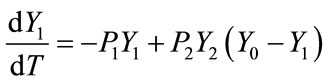 (1a)
(1a)
 (1b)
(1b)
where ,
,  and
and  are positive adjustable parameters associated with the release of charges from traps, retrapping and the charge and electron-hole recombinetion process, respectively. In general the energy dissipation of the recombination process occurs through a radiation process. Thus, the function
  presented in Equation (1) is proportional to the luminescence in crystal phosphor and
  is the concentration of traps [1].
Previous research findings have shown that the solutions for the non-linear stability analysis of equations 1a and 1b are stable, following a hyperbolic path [18]. Mizukami et al. [19] observed that these solutions can be represented by the sum of two terms. The first term leads to slow first order decay and the other to a fast decay. Based on these observations they have proposed an approximate method to reach stable solutions. To obtain the exact solutions, iterative methods can be applied. A family of explicit and implicit iterative methods that has been frequently used are the Runge-Kutta methods [20-22].
In this paper we initially report numerical analyses of the fourth order Runge-Kutta method as applied to the solution of Adirovitch model Equations (1a) and (1b). Even though the RK method is stable, we identified a disconcerting property that emerges from the stiffness of the method when solving these equations: the numerical results are reliable and efficient only for a limited range of parameter values. To solve this problem, this paper proposes an algorithm to determine the best values for parameters in the Runge-Kutta method in order to guarantee the reliability of the results while using the smallest numbers of steps to reach a solution. This algorithm was implemented and has been used in different situations with different parameters. Thus far, to the best of our knowledge, the proposed algorithm has not produced any incorrect solutions.
The paper is organized as follows: in the first section we present the numerical analysis of the Adirovitch model; next, we present the problem of calculating the smallest number of steps to find the solution of this model using a Runge-Kutta Method; and finally we present an algorithm, together with its implementation and tests, to optimize the calculation of the smallest noncritical number of steps to reach the solution.
2. Numerical Analysis
To numerically solve the Equations (1a) and (1b) for the Adirovitch model presented in the introduction of this work it is necessary to find the correct values for each adjustable parameter ,
,  , and
, and . Powerful genetic [23] and statistical [24] methods were developed recently and can be applied in fitting these parameters. Also, other classical methods for fitting can be adopted [25,26]. Nevertheless, fit methods may use a high number of iterations, and the number of steps used for the integration method may increase the computational cost. They may also require large adjustable parameter values. In this context, the solution of Equations (1) using the RungeKutta method, according to the parameters given, may require a large number of steps. Furthermore, the stiffness of the method can create difficulties in the numerical integration of Equations (1) resulting in abnormal and numerically unstable solutions. In this section we will examine the chaotic behaviours of these solutions. In the next section, we propose an algorithm to overcome them.
Equations (1) are made more tractable by introducing the transformations:
 (2)
(2)
where  is the total concentration of trapped charges at the initial instant
 , and
, and . Since the parameters
 ,
,  and
and  enter linearly in the right hand side of Equations (1), mathematically only two of them are really independent. Therefore, it is natural to make an additional scaling. Then, using
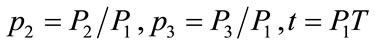 , we deal with only two parameters. Thus, Equations (1) are written as:
 (3a)
(3a)
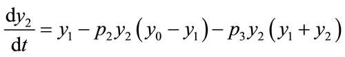 (3b)
(3b)
Numerical methods for the solution of Equations (3) can be divided into two categories [27]. One is the initial value problem, in which the values of  are known at an initial time
 , with
 , requiring the evaluation of
 . The other is the boundary condition for two points, in which boundary conditions are given for
  and
and , typically.
The numerical solution of Equations (3) belonging to the first category are mostly grouped as Runge-Kutta [21, 22,27-30], Bulirsch-Stoer [31], predictor-corrector [32] solutions among others [33,34].
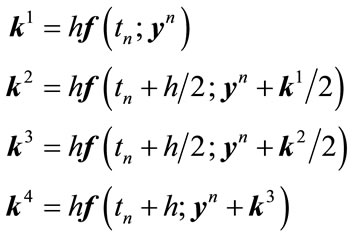
A widely used form of the Runge-Kutta method is of the fourth order. Using a vector notation typical in differential equations,  and
and  , the advancing formula
  from time
  to
to  is given by:
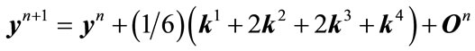 (4)
(4)
where  is the time increment for N steps in which the interval is divided,
The precision of  is proportional to
 . For orders greater than four, it is necessary to evaluate M to M + 2 more functions, increasing the computational cost. The equilibrium between computational efficiency and cost has been found for the fourth order Runge-Kutta method [13,23].
As the error is proportional to , the Runge-Kutta method has a strong dependence on the number of steps. It predicts that the solution is invariant for large numbers of steps and that errors accumulate with any decrease in the number of steps.
Because of the dynamic nature of the Equations (3), it is possible that the accumulation of error makes the solutions erratic. Therefore, we investigated the types of errors that can happen depending on the number of steps and the values of the parameters of the Equations (3).
We have found at least four types of erratic solutions for Equations (3), which are shown in Figure 1. Here we assume that all charge traps are filled ( ) and have no free charges at first (
 ). The time interval used for all calculations in the present work is
 . Figure 1(a) shows an error in which the solutions behave as expected for the exact solutions but whose values are wrong. Figure 1(b) shows deformation errors in which the solution has anomalous depressions or elevations. Figure 1(c) shows an error in which solutions are duplicated, suggesting chaotic behavior. Finally, Figure 1(d) shows erratic solutions leading to divergence. Erratic solutions such as divergence, doubling and deformations are easily identified. Nevertheless, wrong solutions are more difficult to identify.
The existence of incorrect solutions can be evaluated by analysing the correction for the n-th step given by . Figure 2 shows
  as a function of
  in the interval
 , with
 , initial parameters
 ,
,  and (a)
 , (b)
, (b) , (c)
, (c) , and (d)
 . Solid lines linking the values obtained at each i-th step makes the visualization of the properties of
  easy.
easy.
In Figure 2(a) ( ) it is possible to see that the modulus of differences decreases at each step and grows slowly with the increase of
 . This behaviour changes starting at
 , where oscillations can be seen. In Figure 2(b) (
 ) a stranger fin-like formation appears at approximately
 , at the same time that the differences become erratic. In Figure 2(c) (
 ) the fin-like formation appears around
  and doubling appears in
 . In the interval between the beginning of the fin-like formation and the beginning of the doubling, the solutions are incorrect. In Figure 2(d) (
 ), we observed three critical points, one at the fin-like formation (
 ), the second at the doubling (
 ), and the other at a point where the solution diverges completely (
 ). The differences show the appearance of incorrect fin-like, doubling, and divergence type solutions, but they do not allow for prediction
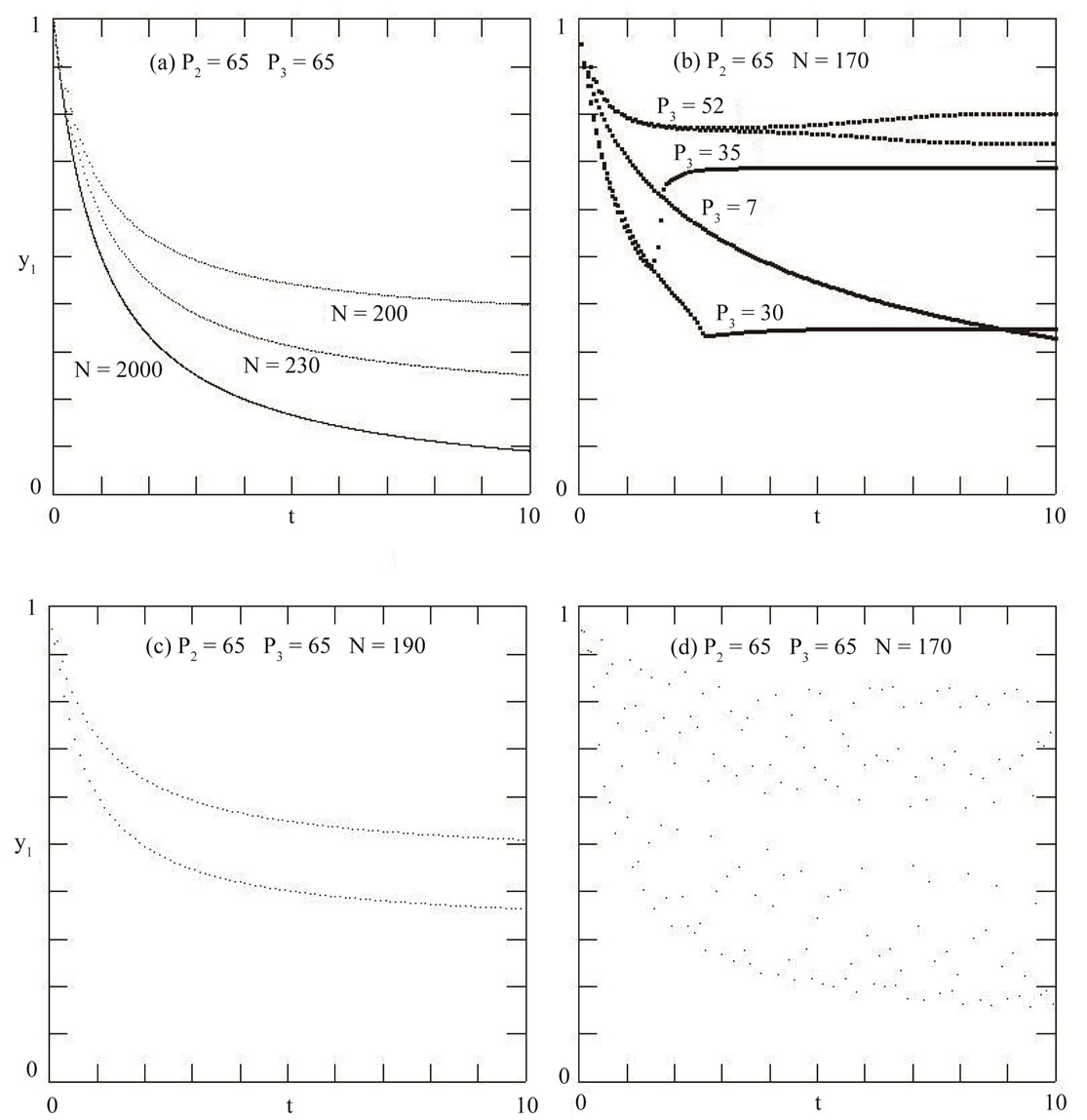
Figure 1. Solution y1 of Equations (3) using the Runge-Kutta method.
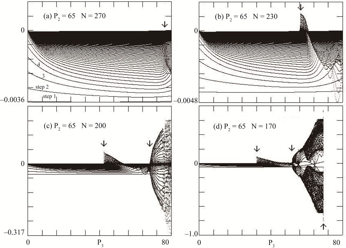
Figure 2. Plot of  as function of
 , with
 , and (a)
 ; (b)
; (b) ; (c)
; (c) ; and (d)
 .
.
of the result of the sum of these differences. In fact we verified through an exact numerical solution of Equations (3) that wrong solutions for N = 170, 200, 230 and 270 begin at approximately , respectively. Therefore,
  is not capable of revealing cumulative errors and a new algorithm must be considered in order to do so.
3. An Algorithm to Optimize the Calculation of the Number of Steps in the Runge-Kutta Method
The analysis given in Section 2 reveals that the Equations (3) behave chaotically depending on the number of steps. Previous research findings have tried to provide mathematical explanations for why such phenomena occur in nonlinear systems [35]. Our work does not intend to build upon these mathematical explanations. Instead, this work intends to create an algorithm that calculates the smallest number of steps necessary to solve the Equations (3), thereby preventing users/programs from encountering these chaotic behaviours. Along these lines, Hagebeuk and Kivits have presented an algorithm in the form of expansion of a very small parameter  to overcome the problem of stiffness [35]. More recently, a new improved class of RK methods of the fourth order were applied with success in several sample problems [36-38]. Nevertheless, the problem of finding the smallest number of steps in which the solutions of RK methods are stable, numerically meaningful and efficiently calculated still remains a subject of great interest [39-42].
3.1. How to Determine the Smallest Non-Critical Number of Steps?
The Runge-Kutta method numerically solves Equations (3) if the solution in a given interval becomes independent of the number of steps (i.e. the number of steps is large enough). However, as discussed in Section 2, we find that  can detect fin-like, doubling and divergence (Figure 2), but cannot show incorrect solutions. This observation is disturbing because it reminds us of the need to perform additional tests to ensure that the number of steps is large enough to give reliable results for the numerical integration. Therefore, we propose an algorithm that executes this task automatically as the solution to find the smallest number of steps to finding a correct solution to Equations (3).
In Section 3, we observed that incorrect solutions may occur from the beginning of the calculations. For example, considering the same interval of integration, for ,
,  , which gives wrong results,
  in the first step is 0.954288... and for
  ,
,  , which gives correct results, it is 0.952203... after 10 steps (the interval is the same in both calculations). This result shows that there is a difference from the beginning of the calculation. On the other hand for N = 2000, p1 = 1, p2 = p3 = 65, the result of the calculation in the first step is 0.995014870675078 and for N = 20,000 after 10 steps the same level of numerical precision is achieved.
By examining these results, we conclude that the result of the application of the RK method using the interval of the first step and dividing it into 10 steps may reveal whether the number of steps will lead to incorrect results. So we will build the algorithm considering only the interval of the first step. We calculate the result of the application of the RK method with a single step in this interval and subtract the result of the calculation obtained by dividing this same interval into M steps. We write this algorithm as:
 (5)
(5)
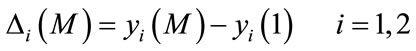
Let us consider the difference  where
where  and
and  are calculated with one and 10 steps in the interval
 , respectively. Then, since we are dealing with an expansion of the fourth order, we expect that to produce a correct solution this difference must be smaller than
 . In case of incorrect solutions, the difference does not maintain proportional to
  and will increase.
Figure 3 shows  as a function of the parameter
 , with
  and the number steps (a) N = 270, (b)
 , (c)
, (c) , and (d)
 . In Figure 3(a) (
 ) the arrow shows a sharp increase in
 , at approximately
 , which coincides with the region where the the results are wrong. In Figure 3(b) (
 ) the arrow shows an abrupt increase in
 , at about
 , which coincides with the fin-like region. In Figure 3(c) (
 ), the first arrow at approximately
 , shows the beginning of a plateau-like region that extends to
 , where the fin-like region indicated by a second arrow begins. In Figure 3(d) (
 ), the first arrow shows the beginning of a plateau-like region extending to
  at about
 , where the fin-like region indicated by a second arrow begins and the third arrow indicates divergence. The plateau-like region is not shown in the plot of
  (Figure 2).
Figure 4 shows the values of  and
and  as a function of the parameter
 , with p2 = 65 and
 . The features of
  and
and  are very similar, until the second arrow; above the second arrow there are differences in the structure of the results. Therefore, the best description of the error in the application of the Runge-Kutta method in the solution of Equations (3) may include both
  and
and  features.
To include the behavior of  and
and , as suggested by the analysis of Figure 4, we chose the last term of equation 1b, because it contains the variables y1 and y2. Therefore we write the new algorithm
  as:
as:
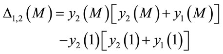 (6)
(6)
Figure 5 shows  as a function of
 , with
  and (a)
 , (b)
, (b) , (c)
, (c) , and (d)
 . Figure 5(a) (
 ) shows agreement with the exact solution until
  , where a sharp increase begins. Figure 5(b)
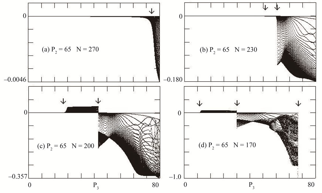
Figure 3. The difference  shown as function of
 , with
 , and (a)
 ; (b)
; (b) ; (c)
; (c) ; and (d)
 .
.
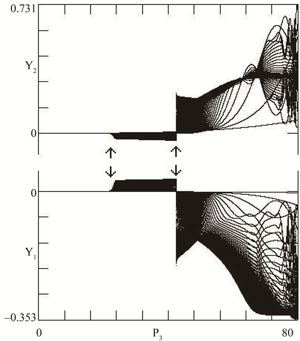
Figure 4. Differences Δ1(10) and Δ2(10) for , with
 , and
, and .
.
( ) shows the exact solution region until
 . Figure 5(c) (
 ) shows the plateau-like region between two arrows. Figure 5(d) (
 ) shows the plateau-like, fin-like and divergence regions successively.
The results of  and
and  are similar for small values of the number of steps (
 and
and ). However when the number of steps increases closer to the number ideal of steps, we observed that
  reveals more details. For this reason, we adopted the algorithm
  to determine the smallest number of steps with which it is possible to reliably solve Equations (3) using the RK method.
Table 1 shows the number of steps and the values of  at the end of the time interval determined using the algorithm
 . For values of parameters
 , we see that the solution for
 , is bifurcated for values equal to or greater than 0.004, but is convergent below 0.0039. We note that in the interval of values of delta between 0.0039 and E-06 the values of steps are equal and the values of
  match up to the third decimal place when compared to the more accurate results. The accuracy in the fifth decimal place is obtained in the interval of E-08 to E-10. For delta equal to E-08, the number of steps is 245 and for E-10 it is 340. For values of parameters
 , we see that the solution is bifurcated for
  values equal to or greater than 0.02. Between 0.01 and 0.019, the solution is wrong. Between 0.004 and 0.001 accuracy is limited to the first decimal place, between 0.0001 and 0.00001 it extends to the third decimal place and for values less than 0.000001 to the fifth decimal place. For delta equal to E-06, the number of steps is 161 and 677 for E-10. In any case, we find that, even for very small values of delta, the magnitude of the number of steps is in an acceptable range of values.
3.2. The Algorithm
Taking into account the above considerations, we propose a 5-step algorithm to determine the smallest noncritical number of steps of the Runge-Kutta method
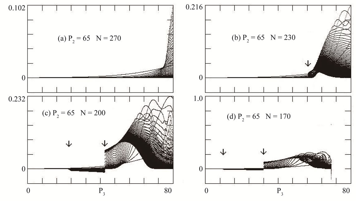
Figure 5. The  difference shown as a function of
 , with
 , and (a)
 ; (b)
; (b) ; (c)
; (c) ; and (d)
 .
.
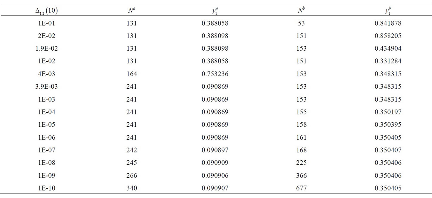
Table 1. Values of the number of steps and the y1 at the end of the time interval determined using the algorithm  with values equal or smaller that those shown in the first column. Values of Na and
  were determined for
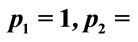
 and of Nb and
  were determined for
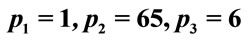 .
.
applied to Equations (3), as follows:
• 1) Define the starting number of steps (50 in the present case);
• 2) Evaluate  using Equation (6);
• 3) Compare  with the minimum acceptable error (E–10 in the present case);
• 4) If  does not match the minimum acceptable value, steps 2 and 3 are repeated with the number of steps increased by a constant value (50 in the present case);
• 5) If  matches the minimum acceptable value, the process is stopped.
Applying the algorithm described above in the example presented in Section 3.1 for , we obtain
  as the smallest non-critical number of steps. The last value calculated for
  in this case (N = 340) is 9.0907128174813E-02, while for
  it is 9.09071645004228E-02. Therefore the number of steps determined by our algorithm gives a solution that is correct and obtains a good degree of accuracy compared with that obtained using a larger number of steps.
To test our algorithm, we implemented a function using the programming language Basic. Part of the code is shown on Table 2. Lines 1 to 14 represent the first step of the algorithm, lines 15 to 33 the second step, lines 34 and 35 the third step, 36 to 40 the fourth step and 41 to 46 the last step. We performed a series of tests changing the parameters of the equations and checking the solution for Adirovitch’s model. To the best of our knowledge, our algorithm has produced only correct solutions.
It is worth noting that we also successfully used the same algorithm to calculate the minimum number of steps to find the correct solution to more complex equations that describes the kinetics of atomic hydrogen [43]. We are aware of other solutions for problems in the Runge-Kutta method [38,39,42,44]. Nevertheless, some of them are not open source (e.g. algorithm presented in MathLab) and others cannot be applied in our previously developed programs and algorithms without extensive changes.
We are currently developing software to simulate and fit the experimental results of decay to time and thermoluminescence using the present algorithm for determining the number of steps, optimizing the parameters using the grid method described in previous work [27]. Preliminary results show perfect integration among these, with safety and manageability.
4. Conclusions
The calculation of solutions for differential equations can be complex and time consuming, requiring large amounts of computational resources (processing time, memory, etc). Thus, it is essential to optimize this process in order to get faster results. In this paper we were interested in using the Runge-Kutta method to calculate the correct solution for the Adirovitch model that uses coupled rate differential equations to describe the kinetic electron trapping process in a shallow defect state and its subsequent thermalor photo-stimulated promotion to a conduction band followed by recombination in another defect.
A series of experiments were carried out, demonstrat-
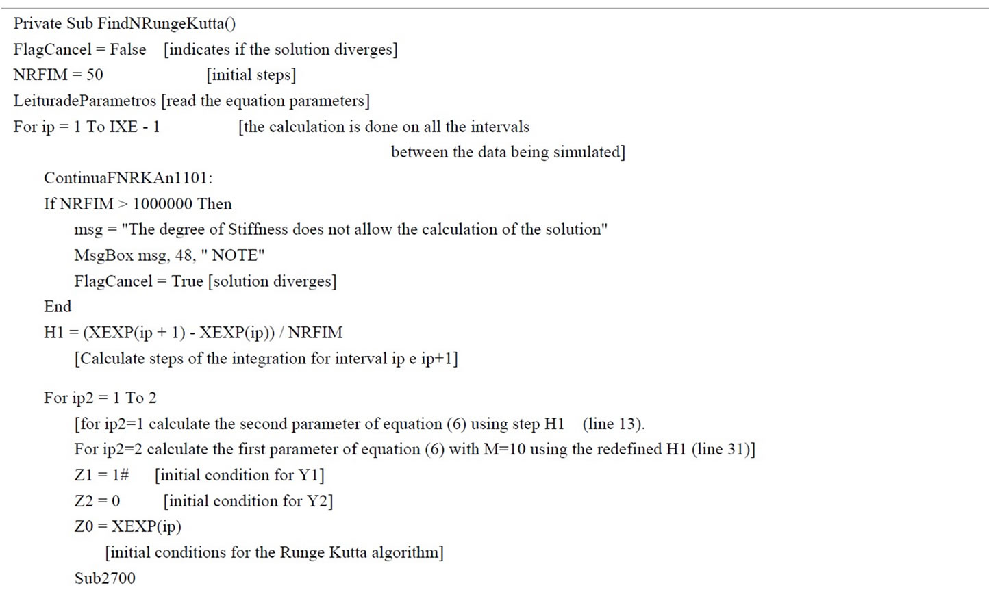
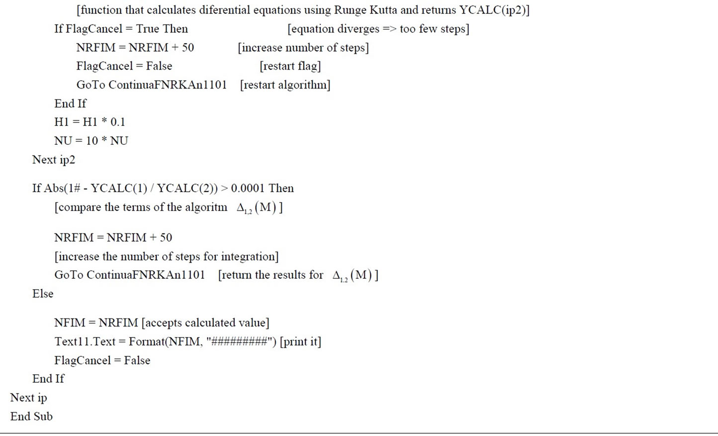
Table 2. Part of the code of the proposed algorithm implemented in Basic.
ing that using the Runge-Kutta Fourth Order method to calculate the solution for the Adirovitch model’s differential equations may lead to incorrect results when the numbers of steps to calculate the solution is not “large enough”. Thus, a numerical analysis was conducted. As a result we develop an algorithm that automatically determines the smallest non-critical number of steps that optimize the calculation of correct solutions of differential equations that follow the same behaviour found in the Adirovitch model. The algorithm is composed of 5 steps: 1) Define the starting number of steps; 2) Evaluate  using Equation (6); 3) Compare
  with the minimum acceptable error; 4) If
  does not match the minimum acceptable value, steps 2 and 3 are repeated with the number of steps increased by a constant value (50 in the present case); 5) If
  matches the minimum acceptable value, the process is stopped. This algorithm was implemented and tested with different values and parameters. We also successfully used the same algorithm to optimize the calculation of more complex equations that describe the kinetics of atomic hydrogen [43].
In future work we will extend this algorithm to support fast calculation of different models that describe physical behaviors using differential equations. We will also use the results of this work to create software that works as a platform to conduct experiments that simulate the behaviors of different models. It will enable users to change the values of parameters in the equations and rapidly check the implications in the behavior of each model.
5. Acknowledgements
This work was supported in part by grants from FINEP, CNPq and FAPESP.
REFERENCES
- E. I. Adirovitch, “The Formula of Becquerel and the Elementary Decay Law of Luminescence of Crystal Phosphors,” Journal of Physique Archives (Paris), Vol. 17, No. 8-9, 1956, pp. 705-707. doi:10.1051/jphysrad:01956001708-9070500
- S. W. S. McKeever and R. Chen, “Luminescence Models,” Radiation Measurements, Vol. 27, No. 5-6, 1997, pp. 625-661. doi:10.1016/S1350-4487(97)00203-5
- C. M. Sunta, W. E. F. Ayta, R. N. Kulkarni, T. M. Piters and S. Watanabe, “Theoretical Models of Thermoluminescence and Their Relevance in Experimental Work,” Radiation Protection Dosimetry, Vol. 84, No. 1-4, 1999, pp. 25-28. doi:10.1093/oxfordjournals.rpd.a032730
- S. Isotani, W. W. Furtado, R. Antonini and O. L. Dias, “Line-Shape and Thermal Kinetics Analysis of the Fe2+- Band in Brazilian Green Beryl,” American Mineralogist, Vol. 74, No. 1, 1989, pp. 432-438.
- R. Antonini, S. Isotani, W. W. Furtado, W. M. Pontuschka and S. R. Rabbani, “Study of the Decay Kinetics of Irradiation Induced Green Color in Brazilian Spodumene,” Proceedings of the Brazilian Academy of Sciences, Vol. 62, No. 1, 1990, pp. 39-43.
- A. S. Ito and S. Isotani, “Heating Effects on the Optical Absorption Spectra of Irradiated, Natural Spodumene,” Radiation Effects and Defects in Solids: Incorporating Plasma Science and Plasma Technology, Vol. 116, No. 4, 1991, pp. 307-314. doi:10.1080/10420159108220737
- S. Isotani, A. T. Fujii, R. Antonini, W. M. Pontuschka, S. R. Rabbani and W. W. Furtado, “Luminescence Study of Spodumene,” Proceedings of the Brazilian Academy of Sciences, Vol. 62, No. 2, 1990, pp. 107-113.
- S. Isotani, W. W. Furtado, R. Antonini, A. R. Blak, W. M. Pontuschka, T. Tomé and S. R. Rabbani, “Decay Kinetics Study of Atomic Hydrogen in a-Si:(H,O,N) and Natural Beryl,” Physical Review B, Vol. 42, No. 10, 1990, pp. 5966-5972. doi:10.1103/PhysRevB.42.5966
- M. B. Camargo, W. M. Pontuschka and S. Isotani, “Electron Paramagnetic Resonance of Atomic Hydrogen Centers in Rubellite,” Proceedings of the Brazilian Academy of Sciences, Vol. 59, No. 1, 1987, pp. 293-298.
- A. R. Blak, W. M. Pontuschka and S. Isotani, “Electron Paramagnetic Resonance of Hydrogen Centers in Natural Beryl,” Proceedings of the Brazilian Academy of Sciences, Vol. 60, No. 1, 1988, pp. 9-12.
- S. Sciortino, “Growth, Characterization and Properties of CVD Diamond Films for Applications as Radiation Detectors,” La Rivista del Nuovo Cimento, Vol. 22, No. 10, 1999, pp. 1-89. doi:10.1007/BF02872270
- T. Budinas, A. Jankauskas, P. Mackup and A. Smilga, “Charge Transport Peculiarities in Thin-Layer Photodielectric System As2Se3Tlx-Sb2S3,” Thin Solid Films, Vol. 36, No. 2, 1976, pp. 277-280. doi:10.1016/0040-6090(76)90021-3
- A. E. do Nascimento, P. Trzesniak, M. E. G. Valerio and J. F. de Lima, “On the Error in the Activation Energy Obtained by the Initial Raise Method for Thermally Stimulated Processes in Dielectrics,” Radiation Effects and Defects in Solids: Incorporating Plasma Science and Plasma Technology, Vol. 134, No. 1-4, 1995, pp. 147-152. doi:10.1080/10420159508227202
- A. Opanowicz, “Interactive Kinetics in Thermally Stimulated Luminescence in Insulators and Semiconductors,” Physica B: Condensed Matter, Vol. 271, No. 1-4, 1999, pp. 273-283. doi:10.1016/S0921-4526(99)00208-2
- L. Brizhik, F. Musumeci, A. Scordino and A. Triglia, “The Soliton Mechanism of the Delayed Luminescence of Biological Systems,” EPL (Europhysics Letters), Vol. 52, No. 2, 2000, pp. 238-244. doi:10.1209/epl/i2000-00429-5
- R. Biswas and B. C. Pan, “Defect Kinetics in New Model of Metastability in a-Si:H,” Journal of Non-Crystalline Solids, Vol. 299-302, Part 1, 2002, pp. 507-510. doi:10.1016/S0022-3093(01)00961-9
- A. D. Drozdov, J. De C. Christiansen, R. Klitkou and C. G. Potarniche, “Effect of Annealing on Viscoplasticity of Polymer Blends: Experiments and Modeling,” Computational Materials Science, Vol. 50, No. 1, 2010, pp. 59-64. doi:10.1016/j.commatsci.2010.07.007
- W. W. Furtado, T. Tomé, S. Isotani, R. Antonini, A. R. Blak, W. M. Pontuschka and S. R. Rabbani, “Numerical Integration Method Applied to the Study of Atomic Hydrogen in Aluminoborate Glass,” Proceedings of the Brazilian Academy of Sciences, Vol. 61, No. 4, 1989, pp. 397-403.
- A. Mizukami, S. Isotani, S. R. Rabbani and W. M. Pontuschka, “Approximate Solution for Kinetic Differential Equations,” Il Nuovo Cimento D, Vol. 15, No. 4, 1993, pp. 637-645. doi:10.1007/BF02482398
- P. Kelly, M. J. Laubitz and P. Braunlich, “Exact Solutions of the Kinetic Equations Governing Thermally Stimulated Luminescence and Conductivity,” Physical Review B, Vol. 4, No. 6, 1971, pp. 1960-1968. doi:10.1103/PhysRevB.4.1960
- J. C. Butcher, “Runge-Kutta Methods in Modern Computation, Part I: Fundamental Concepts,” Computers in Physics, Vol. 8, No. 4, 1994, pp. 411-415. doi:10.1063/1.168500
- P. Rentrop, “Partitioned Runge-Kutta Methods with Stiffness Detection and Stepsize Control,” Numerische Mathematik, Vol. 47, No. 4, 1985, pp. 545-564. doi:10.1007/BF01389456
- A. Brunetti, “A Fast and Precise Genetic Algorithm for a Non-Linear Fitting Problem,” Computer Physics Communications, Vol. 124, No. 2-3, 2000, pp. 204-211. doi:10.1016/S0010-4655(99)00454-3
- F. Khorasheh, A. M. Ahmadi and A. Gerayeli, “Application of Direct Search Optimization for Pharmacokinetic Parameter Estimation,” Journal of Pharmacy and Pharmaceutical Science, Vol. 2, No. 3, 1999, pp. 92-98.
- P. R. Bevington and D. K. Robinson, “Data Reduction and Error Analysis for the Physical Science,” 2nd Edition, McGraw-Hill, New York, 1992.
- S. Isotani and A. T. Fujii, “A Grid Procedure Applied to the Determination of Parameters of a Kinetic Process,” Computer Physics Communications, Vol. 151, No. 1, 2003, pp. 1-7. doi:10.1016/S0010-4655(02)00692-6
- W. H. Press, B. P. Flannery, S. A. Teukolsky and W. T. Vetterling, “Numerical Recipes in C++: The Art of Scientific Computation,” Cambridge University Press, New York, 1988.
- D. W. Zingg and T. T. Chisholm, “Runge-Kutta Methods for Linear Ordinary Differential Equations,” Applied Numerical Mathematics, Vol. 31, No. 2, 1999, pp. 227-238. doi:10.1016/S0168-9274(98)00129-9
- R. I. Mclachlan, Y. Sun and P. S. P. Tse, “Linear Stability of Partitioned Runge-Kutta Methods,” SIAM Journal on Numerical Analysis, Vol. 49, No. 1, 2011, pp. 232-263. doi:10.1137/100787234
- G. Dimarco and L. Pareschi, “Exponential Runge-Kutta Methods for Stiff Kinetic Equations,” SIAM Journal on Numerical Analysis, Vol. 49, No. 5, 2011, pp. 2057-2077. doi:10.1137/100811052
- J. Stoer and R. Bulirsch, “Introduction to Numerical Analysis,” Springer Verlag, New York, 1980.
- C. W. Cear, “Numerical Initial Value Problems in Ordinary Differential Equations,” Prentice Hall, Upper Saddle River, 1971.
- K. Gurski and S. O’Sullivan, “A Stability Study of a New Explicit Numerical Scheme for a System of Differential Equations with a Large Skew-Symmetric Component,” SIAM Journal on Numerical Analysis, Vol. 49, No. 1, 2011, pp. 368-386. doi:10.1137/090775804
- M. J. Feigembaum, “Universal Behavior in Nonlinear Systems,” Physica D: Nonlinear Phenomena, Vol. 7, No. 1-3, 1983, pp. 16-39. doi:10.1016/0167-2789(83)90112-4
- H. J. L. Hagebeuk and P. Kivits, “Determination of Trapping Parameters from the Conventional Model for Thermally Stimulated Luminescence and Conductivity,” Physica B+C, Vol. 83, No. 3, 1976, pp. 289-294. doi:10.1016/0378-4363(76)90123-6
- A. E. Aboanber, “Stability of Generalized Runge-Kutta Methods for Stiff Kinetics Coupled Differential Equations,” Journal of Physics A: Mathematical and General, Vol. 39, No. 8, 2006, pp. 1859-1876. doi:10.1088/0305-4470/39/8/006
- X. J. Wang and S. Q. Gan, “A Runge-Kutta Type Scheme for Nonlinear Stochastic Partial Differential Equations with Multiplicative Trace Class Noise,” Numerical Algorithms, 2012. (To Be Published). doi:10.1007/s11075-012-9568-8
- H. Yuan, J. Zhao and Y. Xu, “Some Stability and Convergence of Additive Runge-Kutta Methods for Delay Differential Equations with Many Delays,” Journal of Applied Mathematics, Vol. 2012, No. 1, 2012, pp. 1-18. doi:10.1155/2012/456814
- J. S. C. Prentice, “Stepsize Selection in Explicit RungeKutta Methods for Moderately Stiff Problems,” Applied Mathematics, Vol. 2, No. 6, 2011, pp. 711-717. doi:10.4236/am.2011.26094
- M. N. Spijker, “Stepsize Conditions for General Monotonicity in Numerical Initial Value Problems,” SIAM Journal on Numerical Analysis, Vol. 45, No. 3, 2007, pp. 1226-1245. doi:10.1137/060661739
- S. Gottlieb, D. I. Ketcheson and C.-W. Shu, “Strong Stability Preservation Runge-Kutta and Multistep Time Discretizations,” World Scientific Publishing Co., Singapore, 2011. doi:10.1142/7498
- A. Valinejad and S. M. Hosseini, “A Stepsize Control Algorithms for SDEs with Small Noise Based on Stochastic Runge-Kutta Maruyama Methods,” Numerical Algorithms, Vol. 61, No. 3, 2012, pp. 479-498. doi:10.1007/s11075-012-9544-3
- W. M. Pontuschka and S. Isotani, “A Model for the Stabilization of Atomic Hydrogen Centers in Borate Glasses,” Physica B: Condensed Matter, Vol. 404, No. 21, 2009, pp. 4312-4315. doi:10.1016/j.physb.2009.08.032
- D. I. Ketcheson and A. J. Ahmadia, “Optimal RungeKutta Stability Regions,” 2012. http://arxiv.org/pdf/1201.3035v2.pdf
NOTES
*Corresponding author.