Applied Mathematics
Vol. 3 No. 11A (2012) , Article ID: 24752 , 11 pages DOI:10.4236/am.2012.331240
Parameter Estimation in Logistic Regression for Transition, Reverse Transition and Repeated Transition from Repeated Outcomes*
1Department of Epidemiology and Biostatistics, Western University, London, Canada
2Department of Statistics and OR, King Saud University, Riyadh, KSA
3Department of Statistics and OR, Kuwait University, Kuwait City, Kuwait
4Samuel Lunenfeld Research Institute, Mount Sinai Hospital, Toronto, Canada
Email: #mchowd23@uwo.ca, chowdhuryri@yahoo.com
Received May 11, 2012; revised October 24, 2012; accepted November 3, 2012
Keywords: Computer Program; Markov Model; Transition; Reverse Transition; Repeated Transition
ABSTRACT
Covariate dependent Markov models dealing with estimation of transition probabilities for higher orders appear to be restricted because of over-parameterization. An improvement of the previous methods for handling runs of events by expressing the conditional probabilities in terms of the transition probabilities generated from Markovian assumptions was proposed using Chapman-Kolmogorov equations. Parameter estimation of that model needs extensive pre-processing and computations to prepare data before using available statistical softwares. A computer program developed using SAS/IML to estimate parameters of the model are demonstrated, with application to Health and Retirement Survey (HRS) data from USA.
1. Introduction
In recent times, there has been a growing interest in the applications of Markov models in various fields. In the past, most of the work on Markov models dealt with estimation of transition probabilities for first or higher orders. The use of higher order Markov chain models for discrete variate time series appears to be restricted due to over-parameterization and several attempts have been made to simplify the application. In recent years, there has been also a great deal of interest in the development of multivariate models based on the Markov Chains. These models have a wide range of application in the fields of reliability, economics, survival analysis, engineering, social sciences, environmental studies, biological sciences. Muenz and Rubinstein employed logistic regression models to analyze the transition probabilities from one state to another for first order [1]. In a higher order Markov model, we can examine some inevitable characteristics that may be revealed from the analysis of transitions, reverse transitions and repeated transitions. Islam and Chowdhury [2] extended Muenz and Rubinstein [1] model to higher order Markov model with covariate dependence for binary outcomes.
Using Chapman-Kolmogorov equations, Islam and Chowdhury introduced an improvement over the previous methods in handling runs of events which are common in longitudinal data [3]. Without loss of generality, they express the conditional probabilities in terms of the transition probabilities generated from Markovian assumptions. Their proposed model is a further generalization of the models suggested by Muenz and Rubinstein [1] and Islam and Chowdhury [2] in dealing with event history data. The proposed model is based on conditional approach and uses the event history efficiently to take account of unequal intervals in the occurrence of events.
In order to estimate parameters of the model proposed by Islam and Chowdhury extensive pre-processing and computations are needed to prepare the data before one can use the standard available procedures in existing statistical softwares [3]. In this paper we present a SAS program developed using SAS/IML to estimate parameters of the proposed model [4]. The program is demonstrated using the follow-up data on Health and Retirement Survey (HRS) from USA.
2. Model
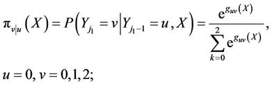
Consider a stationary process  denoting the past and present responses of the i-th subject (
 ) at the j-th follow-up (
 ). Here
  is the response at time
 . One can think of
  as an explicit function of past history of i-th subject at j-th follow-up denoted by
 . The order of the transition model is considered as q, for which the conditional distribution of
  given
given  depends on q prior observations
 .
.
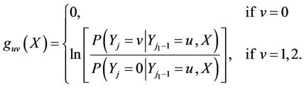
Let us define the multiple outcomes by , s = 0, 1, 2, ···, m−1 if an event of level s occurs for the i-th subject at the j-th follow-up where
  indicates that no event occurs. The first order Markov model can then be expressed as
 , (1)
, (1)
where,  are the m possible outcomes of a dependent variable, Y. The probability of a transition from
  at time
  to
to  at time
  is
is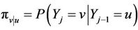 . Note that
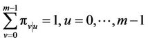 . (2)
. (2)
Figure 1 presents different types of transitions from one state to another state (e.g., state 0 and state 1) for seven hypothetical subjects measured over six consecutive time points for occurrence or non-occurrence of some events (e.g., any disease) without any event at baseline. Subject one has a transition from non-event (0) at time 1 to an event (1) at time 2 and for subject two, the transition took place at time point three. We used  to denote the time of occurrence of transition any time point after first time points. Subject 3 did not make any transition in all six time points, i.e. in other words remained disease free in all six measurements. We can consider it as censored case for transitions Next we consider reverse transition for those subjects who made a transition already. Subject four made a transition from non-event to an event in time 3 and remained in the same state in time 4, after that this subject made a reverse transition from an event to non-event in time point five. The time point of reverse transition is denoted by
 . Subject five remained in state 1 (event) for consecutive follow-ups after making a transition at time point 3 and this we can think as censored cases for reverse transitions.
Finally subjects 6 and 7 are those who already made a transition and a reverse transition and thereafter can only make a repeated transition. Subject six made a transition to event (1) in time point 2 from non-event (0) at time point 1. Then it made a reverse transition at time point 3 to non event. Again at time point 4 this subject made a transition back as event in time point 4, so we called it a repeated transition. Subject seven first made transitions in time 2 then made a reverse transition in time 3 as nonevent and remained in the same state rest of the time points and can be considered as censored for repeated transitions. The time point for repeated transition is denoted by .
.
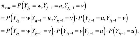
Let us consider m = 3 for illustration of our method. Let the first two states be transient and the third one an absorbing state. For m = 3, we can define the following probabilities using the Chapman-Kolmogorov equations

Figure 1. Flow diagram for different types of transitions.
and also using Equation (1). The probability of a transition from u (u = 0, 1, 2) at time  to v (v = 0, 1, 2) at time
  is
is
 (3)
(3)
where  is the time of follow-up just prior to
 .
.
The probability of a transition from u (u = 0, 1, 2) at time  (just prior to the follow-up at time
 ) to v (v = 0, 1, 2) at time
  (just prior to the follow-up at time
 ) and w at time
  is
is
 (4)
(4)
Similarly, the probability of a transition from u (u = 0, 1, 2) at time  (just prior to the follow-up at time
 ) to v (v = 0, 1, 2) at time
  (just prior to the follow-up at time
 ) to w at time
  (just prior to the follow-up at time
 ) and s at time
  is
is
 (5)
(5)
It is observed that  given in (3), (4) and (5) are initially first, second and third order joint probabilities, respectively. The conditional probabilities may be expressed in terms of first order transition probabilities as:
 (6)
(6)
 (7)
(7)
 (8)
(8)
In the above conditional probabilities (6)-(8), it is assumed that once a transition is made from u to v, then the time of event u will remain fixed for all other subsequent transitions. Here a transition from u to v can happen in the second follow-up or the process can remain in the same state u in consecutive follow-ups before making a transition to v. Similarly, in case of a transition from v to w, the last observed time in state v, before making a transition to w, will remain fixed for any subsequent transition. In other words, we can allow the process to stay in the same state v in consecutive follow-ups prior to making any transition. Finally, if a transition is made from w to s then the process is observed at the last time point in the state of w, before making a transition to s. Here the time of last observing w can be different from the occurrence of w for the first time as found in expressions for  (for the first observed time to transition to w and last observed times for u and v) and
  (for the first observed time to transition to s and last observed times for u, v and w).
Let us define the following notations:
 = vector of covariates for the ith person;
![]()
 = vector of parameters for the transition from u to v.
In what follows we assumes all the individuals start at state u = 0. The probabilities of transition from state u to state v can be expressed in terms of conditional probabilities as functions of covariates as
 (9)
(9)
where
Here,
 .
.
Expressions similar to (9) may be obtained for transition from state v to state w and state w to state s, for details see Islam and Chowdhury and Islam et al. papers [3,5].
3. Estimation
The likelihood function for n individuals with i-th individual having  follow-ups is given by
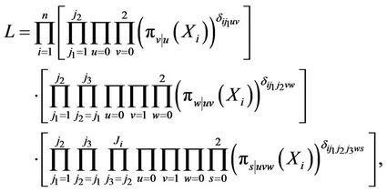 (10)
(10)
and (10) can be expressed as
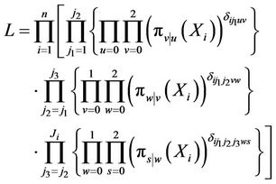 (11)
(11)
where  if a transition type
  (u = 0, v = 1, 2) is observed at
  th follow-up for the ith individual,
  , otherwise;
 , if a transition type
  (u = 0, v = 1, 2) is observed at
  th follow-up and a transition type
  (v = 1, w = 0, 2) is observed at
  th follow-up,
  , if a transition type
  (u = 0, v = 1, 2) is observed at
  th follow-up and a transition type
  (v = 1, w = 0, 2) does not occur at
  th follow-up;
  if a transition type
  (u = 0, v = 1, 2) is observed at
  th follow-up, a transition type
  (v = 1, w = 0, 2) is observed at
  th follow-up, and a transition type
  (w = 0, s = 1, 2) is observed at
  th follow-up,
  , if a transition type
  (u = 0, v = 1, 2) is observed at
  th follow-up, a transition type
  (v = 1, w = 0, 2) is observed at
  th follow-up, and a transition type
  (w = 0, s = 1, 2) does not occur at
  th follow-up.
From (11) the log likelihood function is given by
 (12)
(12)
By equating to zero the derivatives of (12) with respect to the parameters and solving the resulting equations, we obtain the maximum likelihood estimates. The observed information matrix can be obtained from the second derivatives. We can also compute the test statistic for the model as a whole and also for individual parameters [3, 5].
Testing the Global Null Hypothesis
For illustrating the test procedure, let us suppose that all the individuals were in state 0 initially. We will get three sets of parameters, one each for transition, reverse transition and repeated transition. If we consider p variables then  where
where  here
here  are the intercepts, k = 1, 2, 3. Then the likelyhood ratio chi square for testing the null hypothesis
 , is
, is

To test the significance of the q-th parameter of the k-th set of parameters, the null hypothesis is  and the corresponding Wald test statistic is

4. Computations
To explain the computation procedures we will start with a hypothetical data set. Let us consider a binary (0 = no event, 1 = event) outcome variable (i.e. outcome variable with two states) and a single binary covariate (X) from a longitudinal study with 4 follow-ups. We will get three sets of parameters, first one for transition ( ), second for reverse transition (
 ), and a third for repeated transition (
 ). It should be noted that for a multistate outcome variable, number of sets of parameters will increase accordingly [6].
Table 1 gives the hypothetical data on 7 cases. The value of the outcome variable of third follow-up of case 7 (Case ID = 7) is missing and is coded as 99 in the data. Also the value of the outcome variable for this case for the rest of follow-ups will be considered as missing in the data. It should be noted that we have started with only those cases that were in state 0 at follow-up 1. Suppose we have a total of four outcome variables, one for each follow-up. Next we need to find out what are the possible combinations of the values of the outcome variables which will identify the occurrence or non occurrence of an event for transition, reverse transition and repeated transition. Let us explain what we mean by a combination here. For example, case 3 was in state 0 at follow-up 1 and changed its status to state 1 at follow-up 2 (0 → 1). Hence an event took place for this case which we termed as combination (this combination can be viewed like a covariate pattern for four outcome variables from four follow-up) of 0 → 1 and we identified it as a transition [7]. We do not need to worry about the status of this case for follow-up 3 and follow-up 4. If any case remains (e.g., Case 2) in same state for all of the remaining follow-ups as it were in follow-up 1, (0 → 0 → 0 → 0) then this case did not observe any event. Also we have to find out the corresponding covariate value from where a transition or reverse or repeated transition took place.
From the data in Table 1 we have to create three sets of data, one each for say, Set 1 (Transition), Set 2 (Reverse Transition), and Set 3 (Repeated Transition). The created data sets shall include a single binary outcome variable (e.g., “Estatus”) which will identify whether an event occurred (1) or not occurred (0) for each of these three parameter sets and the covariate (X) by taking the value from appropriate follow-ups. In addition we have to create another variable which will identify which cases are for which parameter set (e.g., “TranType”).
To create the new data set with two new variables in addition to the covariates, first we need to identify which cases observed the event for single outcome variable (Estatus) for three sets of data namely Set 1, Set 2, and Set 3. Table 2 shows the possible combination of the value of binary outcome variables of occurrence or non occurrence of events for Set 1 (Transition), Set 2 (Reverse Transition), and Set 3 (Repeated Transitions) with

Table 1. Hypothetical data set with four follow-ups.


Table 2. Combinations of outcome variable for identification of occurrence of events for transition, reverse transition and repeated transitions.
four follow-ups including missing values. There are in total seven possible combinations of outcome variable with four follow-ups (Table 2) for Set 1. First three combinations will identify the occurrence of an event and coded as 1 for the event status column (Estatus). Remaining four combinations will identify the non occurrence of an event for Set 1 and coded as 0 for the event status column (Estatus). Combinations from 5 to 7 with missing values are also considered as non occurrence of an event for Model 1 and are also coded as 0 for the event status column (Estatus). For the first combination in Model 1 for covariate (X) we have to take the corresponding covariate (X) value from follow-up 1, because the event for this transition was originated from followup 1. For combination 2 the corresponding covariate (X) value will be from follow-up 2, and so on. In case of combination four, “no event” was observed. Hence for this case we have to take the covariate value from last follow-up i.e. follow-up 4. For combinations 5 to 6 we have to take the covariate value from first, second and third follow-up, respectively, i.e., the follow-up just prior to the value being missing. The value of transition type (TranType) column is coded as 1 for all of the combinations corresponding to Model 1. Sequence number in (TranCode) column identifies the unique combinations for Set 1.
For Set 2, again we have a total of eight combinations to identify occurrence or non occurrence of events. It is evident that only those cases who observed the occurrence of an event in Set 1 (i.e. made a transition) will be in Set 2 (i.e. can make a reverse transition). First two combinations observed an event (reverse transition) after observing a transition in Set 1 and coded as 1 for the event status column (Estatus) in Set 2. Hence these two combinations will be considered as an occurrence of an event for Set 2. Third to fifth combination in Set 2 did not observe any event after making a transition and will be considered as the non occurrence of an event for Set 2 and coded as 0 for the event status column (Estatus). Sixth and seventh combinations for Set 2 are also considered as non occurrence of an event for this model due to missing observations after making a transition and are also coded as 0 for the event status column (Estatus). The covariate (X) value for Set 2 for first two combinations will be from follow-up 1 and follow-up two, respectively. The covariate (X) value for third to fifth combinations will be from fourth follow-up, since cases with these combinations did not change the state after making a transition. In case of missing data for outcome variable the covariate value for observation six to eight will be from second and third follow-up, respectively. The value of transition type (TranType) column is coded as 2 for all of the combinations corresponding to Set 2. Sequence number in (TranCode) column identifies the unique combinations for Set 2.
Finally for Set 3 (Repeated Transitions) we have five possible combinations from four outcome variables for four follow-ups. Again only those cases who have observed an event for reverse transition will contribute to Set 3. First combination for Set 3 observed an event after observing a transition and then reverse transition, hence is considered as an event for Set 3 (Repeated Transition) or we can say that a repeated transition took place and coded as 1 for the event status column (Estatus). The covariate (X) value for this combination will come from follow-up 3, because the repeated transition was originnated from that point. Second and third combinations did not observe any event after making a reverse transition hence are considered as non occurrence of an event for Set 3 and coded as 0 for the event status column (Estatus) in Table 2. The covariate value for second combination will be from last follow-up as usual and for the third combination will be from third follow-up due to missing value in last follow-up. Fourth and fifth combination will also be considered as non occurrence of event for Set 3 and the corresponding covariate (X) value will come from fourth follow-up. The value of transition type (TranType) column is coded as 3 for all of the combinations corresponding to Set 3. Sequence number in (TranCode) column identifies the unique combinations for Set 3.
Now we can match these combinations of outcome variables of the follow-ups for each case in the data (Table 1) with the combinations for transition, reverse transition and repeated transitions presented in Table 2. For combination 1 in Set 1 (Table 2) we need to match the value for first two follow-ups of the data (Table 1) only. For combination 2 we need to match only with first three follow-ups from the data and so on. Since we created the combinations (Table 2) we can also identify the number of follow-ups to match from the data i.e., the starting follow-up and ending follow-up. For example, for combination 1 in Set 1 the starting follow-up is the first and ending follow-up is the second and so on. Similarly we will be able to identify the appropriate follow-up from where the covariate value should be taken.
Table 3 shows the new data set created by using procedure discussed above for creating data set for Set 1, Set 2 and Set 3. First column in Table 3 (Case ID) gives the case identification. Second column (TranCode) shows which combination was matched by this particular case. Third column (TranType) represents transition types where 1 for transition (Set 1), 2 for reverse transition (Set 2) and 3 for repeated transition (Set 3). Fourth column (Estatus) represents the occurrence or non occurrence of events as discussed earlier. In Set 1 (Transition), five cases observed an event while remaining two did not and coded accordingly in fourth column (Estatus). Those five
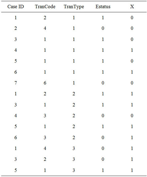
Table 3. Created data set with computed variables.
cases who observed an event in Set 1 can make a reverse transition and are included in Set 2 (see Table 3). Case 1, 3, and 5 observed an event for Set 2 (reverse transition) and 4 and 6 did not observed any event. Finally those who observed a reverse transition (Case ID 1, 3 and 5) can observe only a repeated transition. Two cases (Case ID 1 and 3) did not observed any event after observing a reverse transition (see data in Table 1) and remaining one case (Case ID 5) observed an event for Set 3.
The data set created in Table 3 now can be used to run logistic procedures from statistical software (e.g., SAS, SPSS). Here “Estatus” is the binary dependent variable and X is the covariate. TranType variable is needed to distinguish the three sets of models namely Set 1, Set 2 and Set 3. TranCode variable can be used to run the frequency distribution of different combinations observed in the data set. However, we will need a little more computation to get the overall model test results, since existing statistical software will produce model test separately for three sets of models on the basis of “TranCode” variable.
Algorithm
1) Create all possible combinations on the basis of number of follow-ups for binary outcome variable for transition (Set 1), reverse transition (Set 2) and repeated transition (Set 3).
2) Find the starting and ending follow-up number to for each combination to match with the data.
3) Find covariate(s) position depending on the transition, reverse transition and repeated transition.
4) Match data for each observation with created combination in step 1 by considering appropriate starting and ending follow-up number created in step 2. Create three new variables (TranCode, TranType, and Estatus). Assign appropriate value for each of these three variables.
5) Select the covariate value from the appropriate follow-ups.
6) Create new data set (explained in Table 3) with Case ID, three new created variables (TranType, TranCode and Estatus) and corresponding covariates.
7) Run binomial/multinomial logistic regression using any statistical software (e.g., SAS, SPSS, etc.).
8) Calculate overall model test for all three sets of parameters together.
5. Program Description
As we can see now the estimation of the model parameters is complicated and tedious. In addition it needs to be done in several phases and a large amount of pre-processing for data preparation is needed. We wrote a SAS/ IML function “trrmain()” to make this processing automated. Four arguments have to be provided to invoke the trrmain() function. These are input data file name, number of states for outcome variable, maximum number of follow-ups and number of models for data preparation.
5.1. Input Data File Format
The input data set for our SAS/IML function is needed as a FLAT file format. First variable in the input data file is CASE ID, from 2nd column onward is the outcome variable corresponding to the number of follow-ups. The outcome variable should be coded as 0 and 1 for binary and 0, 1, 2 and so on for multistate (present version of the program will work for binary outcome variable only). Let us consider the hypothetical data provided in Table 1, with four follow-ups; in the input data file second to fifth variables will be the outcome variable and sixth to ninth variable will be the covariate (X), one for each follow-up. If we have another covariate then variable 10 to variable 13 will denote the values of second covariate. The same pattern has to be followed for other covariates, if any. Missing values should be coded as 99 for outcome variables only. However, covariates also may contain missing values and can be left as missing in the data. Table 4 provides a hypothetical sample input data file with two covariates for four follow-ups, where DV is outcome variable and X and Z are two covariates for four followups.
5.2. Sample Run
To demonstrate the use of our program, we have employed data from the Health and Retirement Study (HRS).

Table 4. Input data file format with hypothetical data set for four follow-ups.
The HRS is sponsored by the National Institute of Aging (grant number NIA U01AG09740) and conducted by the University of Michigan (2004). This study is conducted nationwide for individuals over age 50 and their spouses. We have used the panel data from the seven rounds (Health and Retirement Study [8]).
The outcome variable considered here is whether or not an individual were hospitalized during past 12 months for all the rounds. In wave 1, there were a total of 9760 age eligible respondents in the sample (the number was reduced to 9750 due to dropping of 10 cases with missing values of outcome variable at round 1). Finally, we started with 8657 individuals who reported that they were not hospitalized at wave 1. The explanatory variables considered are gender (male = 1, female = 0), number of medical conditions between two consecutive rounds, black (yes = 1, no = 0) and white (yes = 1, no = 0).
The program can be invoked in both SAS 8 and SAS 9. To use our function trrmain(), we need to open the trrmain. SAS file in editor window and run the whole program. Then we need to submit the following SAS statements to INVOKE our function.
proc iml;
load module = trrload;
run trrload;
run trrmain(trdata, 2, 7, 3);
The first argument in trrmain() is trdata which is the SAS data set from input data file. The second argument 2 is for binary outcome variable. The third argument 7 is the total number of follow-ups in our data file. The last argument 3 is for the transition types. If we set the last argument to 1 then it will create data for transitions only, 2 for transition and reverse transitions and 3 for all three models. The newly created data set will be name as “Fdatres” in the SAS WORK library. Our program will use the name for each first follow-up explanatory (e.g., X1, Z1) variable as the explanatory variable name in the newly created data file. Table 5 presents the distribution of occurrence or non occurrence of events (i.e. Estatus variable) from the “Fdatres” data for three models. The program will store a data set named “cmbout” of all possible combinations of outcome variables according to the number of follow-ups with three newly created variables as described in Table 2. Combination of outcome variables from this data can be used as labels for “TranCode” variable.
5.3. Running Logistic Regression from Created Data
Next step is fitting three sets of logistic regression on the basis of TranType variable from “Fdatres” data created by our program and computation of global likelihood ratio test for overall model (all three models together). Following SAS instructions will invoke the logistic procedure.
PROC LOGISTIC COVOUT DATA = Fdatres descending OUTEST = COVM1;
ODS OUTPUT GlobalTests = asts ModelInfo = asts1;
BY TranType;
MODEL Estatus = r1gender r1conde black white;
RUN;
First line of the above instruction invokes logistic procedure and “Fdatres” data set is used. The additional instruction COVOUT and OUTEST = COVM1 adds the estimated covariance matrix to the to Covm1 data set in SAS WORK library for all three models. ODS OUTPUT GlobalTests = asts instruction will store the global test results (Likelihood, Score and Wald) test to asts data set and ModelInfo = asts1 will store model information to asts1 data set in SAS WORK library for all three models separately. There should not be any existing data set with name “covm1”, “asts” and “asts1” in SAS WORK library, if any data in those will be replaced by the above instructions. These we need to compute the overall model test for all the models together. Instruction “BY TranType” will estimate separate models for the three categories of this variable. Left hand side of MODEL statement is the variable for event status as explained earlier and explanatory variables are in the right hand side. Other option can be added to the above instructions (e.g., options for categorical variable). However first two lines should not be changed. Table 6 presents the selected output of logistic regression estimates by the above instructions.
We can use the “SAS/IML” statements to compute the overall model test results as presented in Appendix 1. As the chi-square value for there models stored in “Asts” SAS WORK library, are independent chi-square, we can
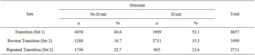
Table 5. Distribution of occurrence or non occurrence of events for three sets.
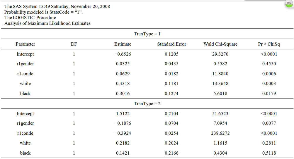

Table 6. Selected SAS output of logistic procedure and overall model test results.
add the chi-square value and degrees of freedom for all the models and compute the new probability. Overall model test results (Log likelihood ratio and Score) are presented in Table 6 (last part). In addition it will also perform the pair wise comparison between three sets (Table 6, last part) of models to see significant differences among them [9,10]. These tests are computed by using necessary information’s from “covm1” and “asts1” data set created by above SAS instructions.
5.4. Mode of Availability
In order to reduce the paper length we did not include the program code here. The full program is available on request. Any one, who is interested, can request the corresponding author for the complete program. The program file and the necessary instruction for users will be sent as e-mail attachment. A hypothetical data set also will be provided for demonstration purpose.
5.5. Limitations
The program has been developed for Markov Models with transient states only. If there is any absorbing state the present version of our program will not work. Also, the present version works only for binary outcome variable. Make sure that there is no data set named “Fdatres” in SAS WORK library; our program will overwrite the existing data set with this name. We are working to extend the program for inclusion of absorbing state [5]. We cannot provide the data set used here according to data use condition from HRS. However, the HRS data products are available to researchers and analysts with appropriate permission. The interested readers can visit the HRS website (http://hrsonline.isr.umich.edu/) for more details about this data set.
6. Conclusion
In this paper we explained the development of SAS/IML program for application to real life data, to estimate the parameters of logistic regression for transition, reverse transition and repeated transition model from follow-up data set. Using the hypothetical data set we have illustrated the algorithm for fitting the model with an application to real data set. Despite the computational complexities, with the use of current state of highly efficient SAS/ IML statements (SAS/IML), the estimates of parameters pose no difficulties. Work is in progress to refine and extend the program for absorbing states and with multistate outcome variable. We hope interested researchers will find it easy to use the function developed by us to estimate the parameters of the model.
7. Acknowledgements
We would like to express our gratitude to the sponsors of the Health and Retirement Survey (HRS) data for allowing us to use the data for our research. The authors acknowledge gratefully to the HRS (Health and Retirement Study) which is sponsored by the National Institute of Aging (grant number NIA U01AG09740) and conducted by the University of Michigan.
REFERENCES
- L. R. Muenz and L. V. Rubinstein, “Markov Models for Covariate Dependence of Binary Sequences,” Biometrics, Vol. 41, No. 1, 1985, pp. 91-101. doi:10.2307/2530646
- M. A. Islam and R. I. Chowdhury, “A Higher-Order Markov Model for Analyzing Covariate Dependence,” Applied Mathematical Modelling, Vol. 30, No. 6, 2006, pp. 477-488. doi:10.1016/j.apm.2005.05.006
- M. A. Islam, R. I. Chowdhury and S. Huda, “A Multistate Transition Model for Analyzing Longitudinal Depression Data,” Bulletin of the Malaysian Mathematical Sciences Society, 2012. http://www.emis.de/journals/BMMSS/accepted_papers.htm
- SAS/IML 9.1, “User’s Guide,” SAS Institute Inc., Cary, 2004.
- M. A. Islam, R. I. Chowdhury and S. Huda, “Markov Models with Covariate Dependence for Repeated Measures, Chapter 9,” Nova Science, New York, 2009.
- M. A. Islam, R. I. Chowdhury and S. Huda, “A Multistage Model for Analyzing Repeated Observations on Depression in Elderly,” Festschrift in Honor of Distinguished Professor Mir Masoom Ali, 18-19 May 2007, pp. 44-54.
- D. W. Hosmer and S. Lemeshow, “Applied Logistic Regression,” Wiley, New York, 1989, p. 136.
- Public Use Dataset, “Health and Retirement Study,” University of Michigan, Ann Arbor, 1992-2004.
- M. A. Islam, “Multistate Survival Models for Transitions and Reverse Transitions: An Application to Contraceptive Use Data,” Journal of Royal Statistical Society A, Vol. 157, No. 3, 1994, pp. 441-455.
- M. A. Islam, R. I. Chowdhury, N. Chakraborty and W. Bari, “A Multistage Model for Maternal Morbidity during Antenatal, Delivery and Postpartum Periods,” Statistics in Medicine, Vol. 23, No. 1, 2004, pp. 137-158. doi:10.1002/sim.1594
Appendix: SAS/IML Code to Compute Overall Model Test Results
proc iml;
reset print;
use Covm1;
read all into xsc;
use Asts;
read all into xsc1;
use Asts1;
read all where(Description=:"Number of Observations") into modsc var{TranType nValue1};
grp=max(xsc1[,1]);
ivar=ncol(xsc)-2;
sconu=do(2,3*grp,3);
loglik=xsc1[(sconu-1),2];
score=xsc1[sconu,2];
nrn=nrow(xsc);
ncn=ncol(xsc);
xsc=xsc[,2:ncn-1];
scon=do(1,nrn,ivar+1);
tcou=0;
do mxg = 1 to grp-1;
co1=xsc[scon[1,mxg],];
sc1=xsc[scon[1,mxg]+1:scon[1,mxg]+ivar,];
nsn1=modsc[mxg,2];
do txg = mxg+1 to grp;
co2=xsc[scon[1,txg],];
sc2=xsc[scon[1,txg]+1:scon[1,txg]+ivar,];
nsn2=modsc[txg,2];
pab=(((nsn1-1)#sc1)+((nsn2-1)#sc2))/(nsn1+nsn2-2);
ch1=(co1-co2)*inv(pab)*t(co1-co2);
chp1=1-probchi(ch1,ivar);
tch=mxg||txg||ch1||ivar||chp1;
tcou=tcou+1;
if (tcou=1) then tch1=tch;
else tch1=tch1//tch;
end;
end;
ch1=sum(loglik);
chp1=1-probchi(ch1,ivar*grp);
ch2=sum(score);
chp2=1-probchi(ch2,ivar*grp);
chn2="Likelihood Ratio"//"Score";
tchim1=ch1||ivar*grp||chp1;
tchim2=ch2||ivar*grp||chp2;
tchim=tchim1//tchim2;
hon1={"Chi-square","D.F","p-value"};
mattrib tchim colname=(hon1) rowname=(chn2) label={'Overall Model Test'} format=f10.6;
print tchim;
ton1={"Model A","Model B","Chi-square","D.F","p-value"};
mattrib tch1 colname=(ton1) label={'Test for Significane Between Different Sets of Estimates'} format=f10.6;
print tch1;
reset print;
quit iml;
NOTES
*Conflict of interest statement: No conflict of interest.
#Corresponding author.