Modern Economy
Vol. 4 No. 3 (2013) , Article ID: 29093 , 16 pages DOI:10.4236/me.2013.43017
Extending the Textbook Dynamic AD-AS Framework with Flexible Inflation Expectations, Optimal Policy Response to Demand Changes, and the Zero-Bound on the Nominal Interest Rate*
1Canadian Economic Analysis Department, Bank of Canada, Ottawa, Canada
2Department of Economics, Amherst College, Amherst, USA
Email: #salpanda@bankofcanada.ca, ahonig@amherst.edu, grwoglom@amherst.edu
Received December 29, 2012; revised January 29, 2013; accepted February 25, 2013
Keywords: Dynamic AD-AS; Inflation Expectations; Optimal Monetary Policy; Liquidity Trap
ABSTRACT
Many popular macroeconomics textbooks have recently adopted the dynamic aggregate demand-aggregate supply framework to analyze business cycle fluctuations and the effects of monetary policy. This brings the textbook treatment much closer to the research frontier, although a major remaining difference is the treatment of inflation expectations. Textbook treatments typically assume adaptive expectations for tractability. In this paper, we extend the model presented in Mankiw [1] by incorporating a more flexible form of expectation formation that is determined as a weighted average of past inflation and the inflation target. This brings the treatment closer to rational expectations and allows for a discussion of costless disinflation. Monetary policy is assumed to follow a Taylor rule, but we allow for deviations from the rule to motivate a discussion regarding optimal monetary policy response to demand shocks. We also include a shock to the risk-premium on the interest rate relevant for demand relative to the policy rate set by the Central Bank, and impose the zero-bound on the nominal interest rate in the solution of the model. These features allow for the analysis of the recent financial crisis, monetary policy falling into a liquidity trap, and the desirability of a temporary increase in the inflation target. Finally, we make available an Excel sheet with which students can analyze the effect of shocks to the economy using impulse responses and dynamic aggregate demand-aggregate supply diagrams.
1. Introduction
For many decades, the teaching of business cycles has been dominated by the investment savings—liquidity money (IS-LM) model whereby monetary policy is summarized using an exogenous level of the money supply (Hicks [2])1. Although this model has served well in many respects, it has often created confusion among students regarding the distinction between deflation and disinflation because of its emphasis on the price level rather than the inflation rate. It has also become less relevant as monetary policy is now typically communicated in terms of a short-term interest rate and, in some cases, a medium-run inflation target.
To overcome these drawbacks, many popular textbooks for undergraduate macroeconomics have recently adopted the dynamic aggregate demand-aggregate supply (DAD-DAS) framework to analyze business cycle fluctuations and the effects of monetary policy (c.f. Jones [4]; Mankiw [1]; Mishkin [5]). The change in the treatment of business cycles found in textbooks has paralleled a burgeoning pedagogical literature that presents alternatives to the traditional Keynesian IS-LM/AD-AS framework that are suitable for undergraduates (Bofinger, Mayer, Wollmershäuser [6]; Carlin and Soskice [7]; Kapinos [8]; Romer [9]; Weerapana [10]; Weisse [11]). These developments have brought the undergraduate treatment of business cycle fluctuations much closer to the research frontier where monetary policy is modeled as an interest rate rule and the analysis is undertaken in the inflation rate-output gap space. At the research frontier, New Keynesian dynamic stochastic general equilibrium (DSGE) models have become the workhorse of business cycle analysis and monetary economics (c.f. Smets and Wouters [12]). In their simplest form, these models can be summarized by three equations: an IS curve relating the output gap to the real interest rate, a Taylor rule summarizing how the nominal interest rate is determined by the Central Bank as a reaction to the prevailing inflation rate and output gap, and finally a Phillips curve expression which relates current inflation to expected inflation and the output gap (c.f. Gali [13]; Clarida, Gali and Gertler [14]). The first two can be combined to obtain an aggregate demand expression in the inflation-output gap space, and the Phillips curve provides the corresponding aggregate supply curve (Kulish and Jones [15]). Although modern variants of these DSGE models feature many layers of complexity, their skeleton is still comprised of these three familiar equations2.
To achieve the leap from the three-equation DSGE model to simpler models suitable for undergraduates found in textbooks and the recent pedagogical literature, several simplifications are used. Most importantly, inflationary expectations are typically assumed to be determined with adaptive expectations (Jones [4]; Mankiw [1]; Carlin and Soskice [7]; Kapinos [8]; Weisse [11]). This has important implications in terms of generating high inflation persistence with temporary shocks and imposing high output costs to disinflationary programs. Also, in this framework, a positive temporary demand shock leads initially to a positive output gap and a rise in inflation, but then several periods of negative output gaps as the adverse effects of higher inflation on the aggregate supply curve continue to reverberate after the positive impact of demand has subsided. Imposing rational expectations would overcome these issues, but would substantially complicate the analysis and is typically ignored.
In this paper, we extend the DAD-DAS model of Mankiw [1] to include a more flexible form of inflation expectations. In particular, we allow inflation expectations to be determined as a weighted average of past inflation and the inflation target. This brings the treatment closer to rational expectations whereby disinflation can be costless if the decrease in the inflation target is credible. This framework also allows us to consider alternative forms of expectations formation simply by changing the weight, with purely adaptive and near-rational (or well-anchored) expectations as the limiting cases.
The paper makes several other contributions to the pedagogical literature on dynamic AD-AS models. First, we include a shock to the risk-premium on the interest rate relevant for demand relative to the policy rate set by the Central Bank. The inclusion of risk shocks is becoming standard in medium-scale DSGE models and allows for a discussion of the recent financial crisis (c.f. Bernanke, Gertler, Gilchrist [18]; Gilchrist, Ortiz, Zakrajsek [19]; Alpanda [20]).
Second, we allow for more flexibility in the way monetary policy is conducted by allowing for deviations from the Taylor rule. Our specification allows for monetary policy to fully offset demand shocks as prescribed by optimal policy (Clarida, Gali and Gertler [14]). It also allows for partial offsetting of demand shocks in the short-run and full offsetting in the long-run, which arguably provides for a more realistic description of actual monetary policy. This partial adjustment in the short-run may capture the unwillingness of the Central Bank to change interest rates too quickly. It could also capture the learning process on the part of the Central Bank regarding the extent of the demand shock. The full-offsetting in the long-run also provides a realistic model of the Central Bank’s response to permanent demand shocks that reinforces the pedagogical point that competent Central Banks can achieve their objectives in the long-run.
Third, we impose a constraint that the nominal interest rate cannot become negative (i.e. the zero-bound on the nominal interest rate). When faced with a large increase in the risk-premium (or a large decline in demand), the Central Bank becomes unable to fully offset this shock due to the zero-bound. We illustrate this liquidity trap situation, faced by the Federal Reserve during the recent financial crisis, using simulations from our model3. We also show how the adverse developments during a liquidity trap (such as negative output gap and possible deflation) can be partially counteracted by the Central Bank by credibly raising the inflation target only temporarily. The temporary increase in the inflation target raises expected inflation and reduces the real interest rate even when the nominal interest rate is stuck at the zero-bound. This reduces the adverse impact of the risk shock on the real interest rate relevant for demand. Note however that the desirability of temporary changes in the inflation target is a point of contention in Central Banks because it could erode the hard-earned credibility of the monetary authority vis-à-vis the long-run inflation target, an issue ignored in our set-up here.
Finally, we make available an Excel sheet with which students can generate impulse response functions of the variables in the model to unexpected shocks and also trace the effects of these developments on a DAD-DAS diagram in the inflation rate-output gap space. We also provide a similar analysis in the unemployment rateinflation rate space using a Phillips curve diagram. Importantly, our Excel sheet allows for simulating the effects of different shocks simultaneously. This enables us to study, among other possibilities, the effects of adverse risk shocks and concurrent changes in the inflation target in order to avoid the liquidity trap4.
The rest of the paper is organized as follows: Section 2 introduces the model. Section 3 discusses the accompanying Excel sheet and explores the main implications of the model. Section 4 concludes.
2. The DAD-DAS Model
The model is based on the DAD-DAS model in Mankiw [1], although with several important modifications. First, we allow a more flexible form of inflation expectations that depends not only on past inflation, but also on the inflation target. Second, on top of demand and cost-push shocks explored in Mankiw [1], we include a shock to the risk-premium which drives a wedge between the policy rate and the interest rate relevant for demand. Third, we allow monetary policy to deviate from the Taylor rule when the economy is hit with demand-type shocks. Fourth, we impose the zero-bound on the nominal interest rate. Finally, we model the persistence of shocks explicitly and consider the effects of permanent as well as temporary shocks to demand.
The demand side of the model is summarized with an IS equation that reads:
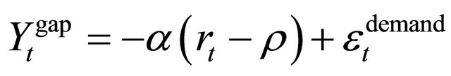 , (1)
, (1)
where  is the output gap defined as the percentdifference between actual output and the natural rate of output.
  is the natural real interest rate capturing the real interest rate in the long-run of the model (which would equal the marginal product of capital minus the depreciation rate in the Solow growth model). This longrun real interest rate is set equal to 2% following Mankiw [1]5.
  is an elasticity parameter capturing the sensitivity of the output gap to changes in the real interest rate, and is set equal to 1 in the benchmark calibration as in Mankiw [1]. When the prevailing ex-ante real interest rate exceeds the long-run natural rate (i.e. when the interest rate gap,
  , is positive), consumption and investment demand are constrained, which results in a negative output gap all else equal.
  is a demand shock where a positive value would generate a higher output gap for the same real interest rate. This captures variation in consumption, investment or government expenditure demand that is not related to the interest rate gap.
The real interest rate that is relevant for the IS relationship above is defined as the difference of the nominal interest rate and expected inflation, plus a risk-premium shock,  , which changes exogenously over time and reflects the wedge between the policy rate set by the central bank and the cost-of-capital and borrowing costs incurred by final demanders6:
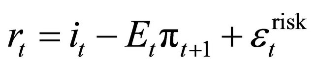 . (2)
. (2)
As shown later, risk shocks affect the economy analogously to demand shocks and move inflation and output gap in the same direction.
The short-run aggregate supply is summarized by a New-Keynesian Phillips curve given by:
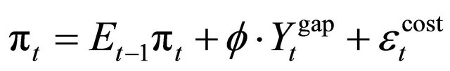 , (3)
, (3)
where current inflation is partly determined by past expectations regarding current inflation (because of predetermined prices)7. The output gap also affects current inflation as higher output results in an increase in the marginal cost of production.  is an elasticity parameter capturing the sensitivity of inflation to changes in the output gap and is set equal to 0.25 in the benchmark calibration following Mankiw [1].
  is a cost-push shock that captures changes in current inflation due to unexpected changes in costs (such as changes in oil prices).
Expectations regarding future inflation are assumed to be based on a mixture of current inflation (capturing adaptive expectations) and the future inflation target of the Central Bank (capturing rational expectations—assuming the target is credible)8:
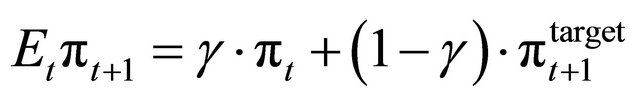 , (4)
, (4)
where  is a parameter that determines the weight on current inflation in generating expectations about the future. If
 , then expectations are fully adaptive. If on the other hand
 , then the expectations are (close to) rational and are based on the inflation target set by the Central Bank.
Monetary policy is summarized by a Taylor rule on the nominal interest rate except when the Taylor rule implies a negative rate in which case the rate is set to 0; hence,
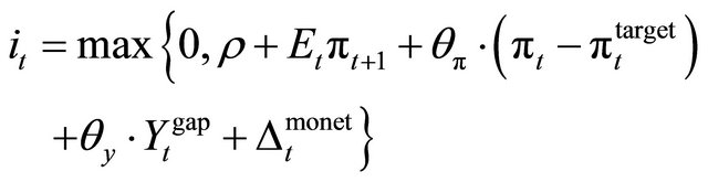 (5)
(5)
 and
and  are response coefficients of the Central Bank to deviations of inflation from its target and the output gap respectively. We set both
  and
and  equal to 0.5 following Taylor [28] and Mankiw [1]. Note that, coupled with the expected inflation term on the righthand-side, the interest rate rule satisfies the Taylor principle that states that the nominal interest rate should be raised more than the increase in expected inflation. This results in an increase in the ex-ante real interest rate and curbs demand when inflation starts to rise. The inflation target is assumed to be initially set at 2% as in Mankiw [1].
 is a term that captures deviations of monetary policy from the Taylor rule9. Note that optimal monetary policy under full-information would recommend fully offsetting demand-type shocks since they move inflation and output gap in the same direction, and therefore, do not entail a tradeoff between inflation volatility and output gap volatility for the Central Bank. This requires monetary policy to be more active than a Taylor rule in order to shift the DAD curve back (as explained later, strictly following the Taylor rule would only provide a movement along the DAD curve which cannot fully offset a demand-type shock). We therefore model this deviation term as follows:
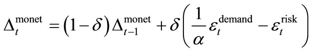 , (6)
, (6)
where  is a parameter that captures the extent to which the Central Bank offsets demand-type shocks (i.e. demand and risk shocks). Setting
  recovers the benchmark case where the Central Bank strictly follows the Taylor rule (given past deviations are zero). With
 , monetary policy fully offsets demand shocks as prescribed by optimal policy (Clarida, Gali and Gertler [14])10. By considering
  to be between 0 and 1, we also allow for partial offsetting of demand shocks in the short-run. Given our lagged deviation term on the right hand side of (6) however, the Central Bank fully offsets demand shocks in the long-run; this arguably provides for a more realistic description of actual monetary policy. This partial adjustment in the short-run may capture the unwillingness of the Central Bank to change interest rates too quickly. It could also capture the learning process on the part of the Central Bank regarding the extent of the demand shocks.
Finally, Okun’s Law summarizes the relationship between the unemployment rate and the output gap as:
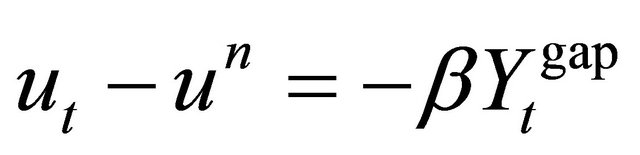 , (7)
, (7)
where the natural unemployment rate,  , is set at 5% and the unemployment rate rises by
  percentage points for every percentage point decline in the output gap. Note that the Okun’s Law expression is not central to the determination of equilibrium of the model; it is merely added here as a side equation that can help translate output gap numbers into, perhaps more intuitive, unemployment rates.
2.1. Persistence of Shocks
We assume that risk and cost-push shocks have only temporary effects on the economy. We nevertheless allow these shocks to possibly persist into the future by modeling them as stationary AR(1) processes:
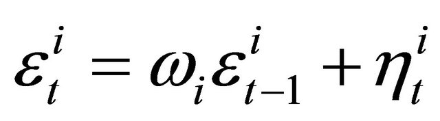 (8)
(8)
where  is the persistence parameter, and
  is the innovation to the shock process for each
 .
.
For demand shocks, we consider the effects of both temporary  and also permanent shocks (i.e.
 ), the latter capturing permanent changes in private savings behavior or permanent changes in fiscal policy. For the inflation target, we assume that any change announced by the Central Bank is permanent in the benchmark case (by setting the number of periods that inflation target, cell C23 in the Excel workbook, to a number equal to or greater than 51). We also allow the change in the inflation target to be temporary, by setting the number of periods that the inflation target is in effect to a number less than or equal to 50.
2.2. Solution of the Model
In this subsection, we first solve the model under the assumption that the zero-bound on the nominal interest rate does not bind. In particular, we derive the dynamic aggregate demand (DAD) and the dynamic aggregate supply (DAS) expressions that characterize equilibrium. We then discuss how the equilibrium is amended to allow for the zero-bound to occasionally bind.
To derive DAD, we first combine Equations (2) and (5) to solve for the interest rate gap:
 . (9)
. (9)
We then plug the above expression into the IS equation in (1) to get:
 (10)
(10)
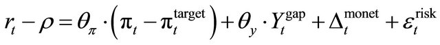
We then rearrange terms and solve for the output gap in terms of current inflation and various shocks. This yields the DAD expression:
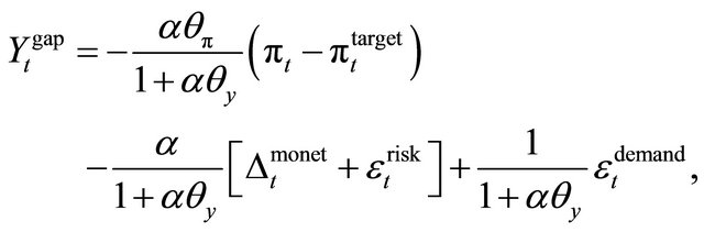 (11)
(11)
which summarizes an inverse relationship between inflation and the output gap. In particular, an increase in inflation prompts the Central Bank to increase the nominal and the real interest rate and cause a reduction in demand. Note that the interest rate is not constant along a DAD curve in this setup. The Central Bank’s reaction to inflation developments according to the Taylor rule results in movements along the DAD curve. Changes in demand and risk shocks (or a deviation from the Taylor rule), result in a parallel shift of the DAD curve.
The slope of the DAD curve is partially determined by the Central Bank’s response coefficients to inflation and output gap in the Taylor rule. A higher , the response coefficient to inflation, or a lower
 , the response coefficient on output gap, is associated with a flatter DAD curve (with inflation drawn on the y-axis) as the Central Bank becomes less tolerant of inflation variation and more tolerant of output gap variation. Note that if the Taylor principle is violated, e.g. if
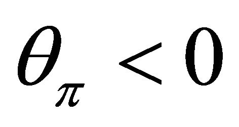 , then the DAD curve becomes upward-sloping.
To derive DAS, first note that the inflation expectations equation (4) implies
 .
.
We plug this into the Phillips curve expression (3) to get the (short-run) DAS expression:
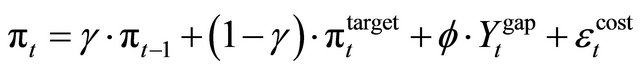 , (12)
which summarizes a positive relationship between inflation and the output gap. Achieving a higher level of production in the short-run comes at the cost of increased marginal costs which feed into current inflation. This is captured through a movement along the DAS curve. Inflation expectations play a crucial role as well since prices are predetermined and are assumed to be “sticky” for a period. Changes in inflation expectations and the cost-push shock result in a shift of the DAS curve.
Note that the shocks and the inflation target are exogenously determined; therefore, the DAD and DAS equations have only two unknowns: the output gap and the inflation rate. We can solve for the equilibrium values of output gap and inflation as the intersection of the DAD and DAS curves, and then derive the nominal interest rate from the Taylor rule and the real interest rate from Equations (2) and (4). This constitutes the equilibrium when the zero-bound on the nominal interest rate does not bind.
General Solution of the Model When the Zero-Bound can Occasionally Bind
To find the general solution when the zero-bound can occasionally bind, we derive equilibrium in an analogous, but perhaps less intuitive fashion. We first set the nominal interest rate to 0 or the equilibrium value found in the previous subsection under the Taylor rule assumption, whichever one is higher. We then use Equations (1)-(4) to solve for the real interest rate,  , in terms of the nominal interest rate, past inflation, and the exogenous variables in the model as:
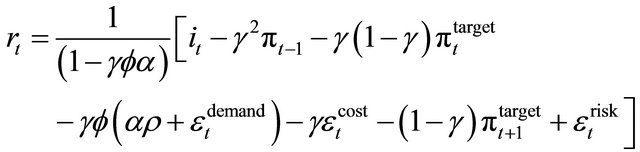 (13)
(13)
Equation (1) then yields the equilibrium value of the output gap and Equations (3) and (4) yield the inflation rate.
When the zero-bound does not bind, the equilibrium obtained here using Equation (13) is equivalent to the equilibrium obtained in the previous subsection under the Taylor rule. The equilibrium values for the endogenous variables would differ though when the zero interest rate binds. Since past inflation is a state variable in the system (i.e. a variable that can affect current values), it is important to always take these past inflation figures from the equilibrium obtained from the general solution—even when calculating the equilibrium under the Taylor rule assumption—during the simulation process in Excel.
3. The Excel Sheet and Main Results
In this section, we explain how the accompanying Excel workbook can be used to simulate the DAD-DAS model presented in Section 2. We provide examples as well as a discussion of issues that relate to inflation expectations and duration of shocks.
3.1. Using the Excel Sheet
The Excel workbook in the worksheet called “Model” contains cells (in column C) for the model’s structural parameters,  , the monetary policy parameters
  (the last one sets the initial inflation target before any possible changes are made), the shock persistence parameters,
  , the share of past inflation in the inflation expectation expression,
  , the share of demand shocks offset by the Central Bank in the short-run,
  , and the number of periods that a change in the inflation target is in effect. All of these parameters can be altered and are highlighted in yellow on the worksheet. The effect of shocks and the inflation target can be analyzed by changing the values of the exogenous variables at time 0 in cells G7:J7, which are also highlighted in yellow.
The structural and policy parameters are set to the same benchmark values as in Mankiw [1].
The model is assumed to be at the steady-state prior to period 0. Period 0 is the impact period when there is an unexpected change in the inflation target or a demand, cost-push, or risk shock hits the economy. The workbook then calculates the future equilibrium values of the endogenous variables, which are also plotted in the worksheets called “Impulse response chart”, “DAD-DAS chart”, and “Phillips curve chart”. The impulse response charts trace the effects of the shock(s) on output gap, inflation and the interest rates over time following the impact period. The DAD-DAS chart captures this dynamic behavior in the output gap-inflation rate space. It plots the initial position of the DAD and DAS curves at the steady-state prior to any shocks and replots these curves with appropriate shifts at the impact period of the shocks. Following these shifts, the diagrams trace out the equilibrium path of output gap and the inflation rate over time using arrows. The Phillips curve chart provides a similar analysis in the unemployment rate-inflation rate space.
3.2. The Effects of Temporary Cost-Push Shocks
In Figures 1 and 2, we present the impulse response and the DAD-DAS charts resulting from a 1 percentage point positive cost-push shock with zero persistence (i.e.
Impulse responses

Figure 1. Impulse responses to a +1% cost-push shock with 0 persistence under fully adaptive expectations.
Dynamic AD-AS
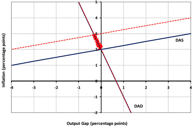
Figure 2. DAD-DAS diagram for a +1% cost-push shock with 0 persistence under fully adaptive expectations.
 ) under fully adaptive inflation expectations (i.e.
 )11. The shock can be simulated by changing the value of cell G7 from 0 to 1. The AS curve shifts up by 1 percentage point which leads to an immediate increase in inflation. This prompts the Central Bank to raise the nominal interest rate by more than 1 percentage point, which raises the real interest rate and causes a decline in the output gap. The resulting negative output gap ensures that the increase in inflation in equilibrium at the impact period is less than 1%. Even though the cost-push shock has no persistence, adaptive expectations ensure that inflation remains above target for a prolonged period of time. Over time, inflation slowly declines back to the target (due to the negative output gap), while the output gap increases back to 0 as the initial interest rates are restored.
Note that the adjustment process is much faster, even immediate, when inflation expectations are not adaptive, but fully based on the inflation target. If we set , then the shock’s effect lasts only for one period, and the economy reverts back to the steady-state immediately after the impact period. When inflation expectations are formed in part in adaptive fashion and in part based on the target (e.g.
 ), then the adjustment process is faster than the case with fully-adaptive expectations, but not immediate.
As argued above, adaptive expectations can result in inflation persistence even when the inflation shock is very temporary12. Alternatively, if the cost-push shock is persistent, it will lead to a prolonged period of high inflation and negative output gaps even when inflation expectations are fully based on the inflation target and are not adaptive at all. For example, the impulse responses for output gap and inflation are similar when  and
and  versus when
  and
and .
.
3.3. The Effects of Temporary Demand (and Risk) Shocks
In this section, we analyze the effects of temporary demand shocks on the economy under two separate assumptions regarding monetary policy. In the first, we assume that the Central Bank follows the Taylor rule and does not deviate from it as in Mankiw [1]. In the second, we allow the Central Bank to partially or fully offset the demand shocks as implied by optimal policy. Our analysis here also extends to risk shocks which are analogous to demand shocks as implied by the DAD expression in (1.10).
3.3.1. Case I: Central Bank Does Not Deviate from the Taylor Rule
In Figures 3 and 4, we present the impulse response and the DAD-DAS charts resulting from a 5 percentage point Impulse responses
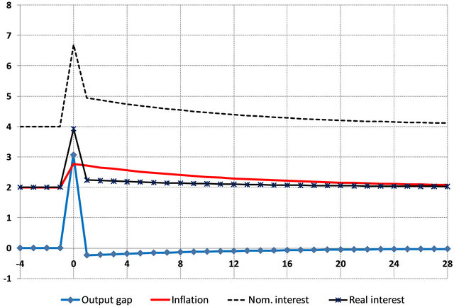
Figure 3. Impulse responses to a +5% demand shock with 0 persistence under fully adaptive expectations and no deviations from the Taylor rule.
Dynamic AD-AS

Figure 4. DAD-DAS diagram for a +5% demand shock with 0 persistence under fully adaptive expectations and no deviations from the Taylor rule.
positive demand shock with zero persistence (i.e. ) under fully adaptive inflation expectations (i.e.
 ) and the Central Bank not deviating from the Taylor rule (i.e.
 ). The shock can be simulated by changing the value of cell H7 from 0 to 5. The AD curve shifts to the right by 5 percentage points which leads to an increase in both the output gap and the inflation rate at the impact period. In equilibrium, the output gap increases less than the initial 5% shift. This is because the Central Bank raises the nominal interest rates above and beyond the increase in expected inflation which leads to an increase in the real interest rate and curbs aggregate demand. Right after the impact period, the demand shock reverts back to 0 and the DAD curve shifts back to its original position. Note however that in this example inflation expectations are fully adaptive. The increase in inflation in the impact period becomes entrenched and therefore causes an upward shift in the DAS curve. This results in a negative output gap and an inflation rate that is higher than target, similar to a cost-push shock, right after the impact period. Inflation slowly goes down to target and output gap slowly recovers to zero as time elapses, as was the case with the cost-push shock examined before.
When inflation expectations are based solely on the inflation target (i.e. ), the model does not generate any negative output gap when hit with a temporary positive demand shock. If the demand shock has no persistence, then the model reverts back to the initial steady-state immediately after the impact period. The reason is that the increase in inflation during the impact period does not feed into future inflation and therefore does not cause any effects on the output gap. If the demand shock is persistent, then the economy goes through periods of above-target inflation and positive output gaps until the effects of the shock die down.
Under fully rational expectations (i.e. with modelconsistent expectations), inflation expectations would increase above target in the short-run if the shock is persistent. Our model cannot simulate fully-rational expectations with persistent shocks. Nevertheless, the impulse responses obtained would be similar if in our set-up we consider a persistent shock (e.g. ) with inflation expectations formed as a combination of past inflation and target inflation (e.g.
 ). Figures 5 and 6 plot the impulse responses from a +5% demand shock given the above numbers for the persistence and expectations parameters. The impulse responses imply that the economy experiences positive output gap along with above-target inflation for a prolonged period of time. During the transition, the DAS curve shifts as inflation expectations are partially affected from past above-target inflation.
3.3.2. Case II: Central Bank Offsets the Temporary Demand Shock
Demand shocks do not pose a tradeoff for the Central Bank as they move both inflation and output gap in the same direction. If the Central Bank is averse to fluctuations in inflation and output gap, optimal policy would suggest that the Central Bank should fully offset all demand shocks [14]. Note that the Taylor rule utilized by the Central Bank cannot achieve this automatically. As shown in Figures 3 and 5, the Taylor rule indeed recommends an increase in the nominal and real interest rates as a result of a positive demand shock. This ensures that the increase in the output gap is less than the 5 percentage point shift considered. Note however this is merely a movement along the new DAD curve and does not shift the DAD curve back.
As the Central Bank becomes aware of the presence of a positive demand shock, it could do more than the Taylor rule (i.e. it could increase the interest rates more than the Taylor rule to shift the DAD curve back faster). In Impulse responses
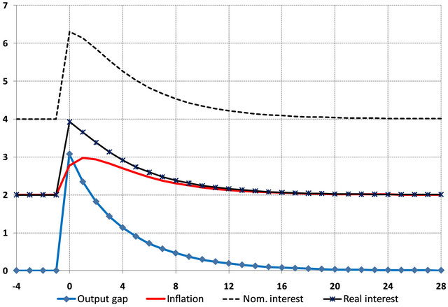
Figure 5. Impulse responses to a +5% demand shock with 0.8 persistence and inflation expectations parameter = 0.5 and no deviations from the Taylor rule.
Dynamic AD-AS
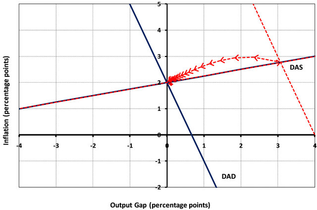
Figure 6. DAD-DAS diagram for a +5% demand shock with 0.8 persistence and inflation expectations parameter = 0.5 and no deviations from the Taylor rule.
our set-up, this could be obtained by setting the parameter relating to the deviation from the Taylor rule, δ, to a value greater than 0. For illustration, we first set this parameter equal to 1 to capture full-offsetting of demand shocks by the Central Bank and consider the same demand shock as before (see Figure 7). As shown, both the output gap and inflation stay at their initial steady-state position without any change, but the nominal and real interest rates rise in order to offset the effects of the demand shock13. It may be more realistic to assume that the Central Bank would choose to offset demand shocks slowly as it may be unwilling to change interest rates too quickly or may need more time to fully grasp the extent of the demand shock. This gradual offsetting of demand shocks by the Central Bank can be captured by setting  to a value between 0 and 1.
3.4. The Effects of Permanent Demand Shocks
In this section, we extend our previous analysis to permanent demand shocks. Note however that what we discuss here is also relevant for temporary, but very persistent, demand shocks as well.
In Figures 8 and 9, we explore the effects of a 1% permanent increase in demand (which may be as a result of a permanent change in the savings attitudes of households or a permanent change in fiscal policy). Under fully adaptive expectations and the Central Bank strictly following the Taylor rule, the model generates the counterintuitive and incorrect result that the long-run inflation rate is permanently increased as a result of the demand shock. This is despite the fact that there has been no change in the inflation target. The output gap gradually converges to 0 and the real interest rate is permanently increased. The latter is consistent with the Solow growth model’s implication that a permanent decline in the overall savings rate would result in a decline in the capital-output ratio and an increase in the real interest rate at the new steady-state and along the transition path. The inconsistency arises from the model’s implication regarding long-run inflation.
In our framework, this can be amended by considering a gradual offsetting of the demand shock by the monetary authority (see Figure 10). The deviation from the Taylor rule results in a quicker convergence of the output gap to zero and inflation gradually converges back to the target rate of 2%. The real interest rate gradually rises to a permanently higher level as a result of the permanent decline in savings, which also results in a permanent increase in the nominal interest rate.
3.5. Permanent Changes to the Inflation Target and Costless Disinflation
Suppose the Central Bank decides to permanently lower its inflation target to 1%. To simulate this change in the Excel workbook, the value in cell J7 is changed from 2 to Impulse responses
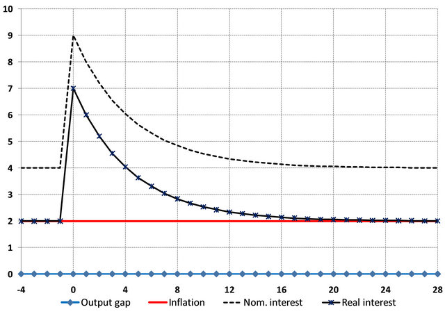
Figure 7. Impulse responses to a +5% demand shock with 0.8 persistence when the Central Bank fully offsets the demand shock (inflation expectations parameter = 0.5).
Impulse responses

Figure 8. Impulse responses to a +1% permanent demand shock under fully adaptive expectations and no deviations from the Taylor rule.
Dynamic AD-AS
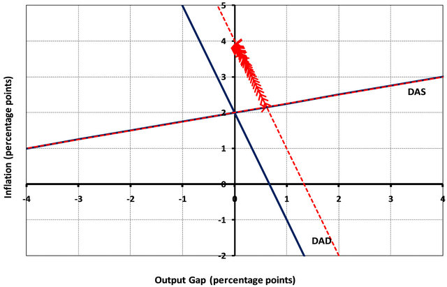
Figure 9. DAD-DAS diagram for a +1% permanent demand shock under fully adaptive expectations and no deviations from the Taylor rule.
Impulse responses

Figure 10. DAD-DAS diagram for a +1% permanent demand shock under fully adaptive expectations and with gradual offsetting of the shock by the Central Bank (δ = 0.5).
1. Figures 11 and 12 show the resulting impulse responses under the assumption of fully-adaptive inflation expectations (i.e. ) and expectations that are fully based on the inflation target (i.e.
 ), respectively13. When expectations are adaptive, the change in the inflation target results in a period of negative output gaps along with falling inflation. Since at the time of impact, current inflation (which is close to 2%) is higher than target inflation (equal to 1%), the Central Bank raises the nominal interest rates to reduce demand, which causes the negative output gap. This reduces inflation over time, but the decrease of actual inflation to the target is gradual due to adaptive expectations, and the disinflation process therefore is costly in terms of foregone output. Over timeImpulse responses

Figure 11. Impulse responses to a permanent decrease in the inflation target from 2% to 1% under fully adaptive expectations.
Impulse responses
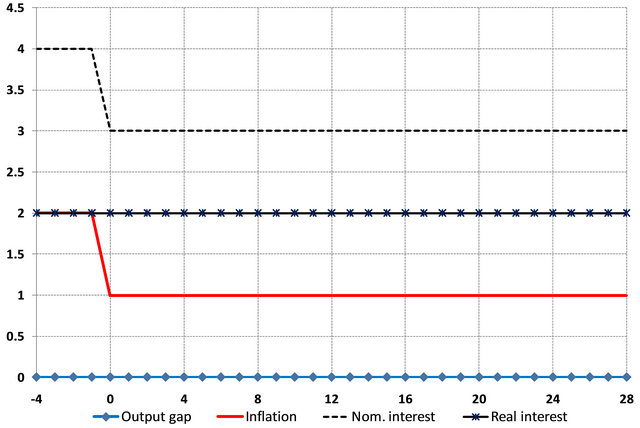
Figure 12. Impulse responses to a permanent decrease in the inflation target from 2% to 1% under inflation expectations fully based on the credible inflation target.
the nominal interest rate declines along with the decline in the inflation rate (i.e. the Fisher effect). On the other hand, when expectations are based fully on the (credible) inflation target, the disinflation process is costless in terms of the output gap. Both the inflation rate and the nominal interest rate decline by 1 percentage point immediately as a result of the change in the inflation target, but this does not cause any changes to the real interest rate or the output gap.
3.6. The Zero-Interest Rate Bound and the Liquidity Trap
As Equation (1.9) indicates, the effects of risk-shocks on inflation and the output gap are analogous to demand shocks. We have included them in our model separately though to point out that the real interest rate implied by Central Bank policy may not reflect the real interest rate relevant for demand. More importantly, there may be times, as in the recent financial crisis, when the increase in risk-premia may result in an increase in the real interest rate relevant for demand despite the decline in the nominal interest rate set by the Central Bank.
In principle, the Central Bank can fully offset the effects of risk shocks with a larger change in the policy rate called for by the Taylor rule. In particular, if the risk shock increases by 7% and shifts the AD curve to the left, immediately lowering the nominal interest rate by 7 percentage points would shift the DAD curve immediately back to its initial position (with no resulting change in the output gap or inflation). A problem arises however if the nominal interest rate cannot be lowered by the full 7 percentage points due to the zero-interest rate bound, a situation known as the “liquidity trap”. A full offsetting of the risk shock cannot be achieved in this case and the best that the Central Bank can do is to lower the nominal interest rate to 0. Thus, the economy cannot escape a high real interest rate (including the risk-premium) and a corresponding negative output gap situation even when the Central Bank immediately recognizes and tries to fully offset the risk shock (see Figure 13).
During the recent financial crisis, there were discussions regarding temporarily increasing the target inflation rate by a few percentage points. This was intended to reduce the downside risks involved with deflation, lower real interest rates even when the nominal interest rate is stuck at 0, and slow down the decline in nominal asset prices. The latter was thought to be crucial in order to provide relief to homeowners with negative equity in their homes due to the decline in housing prices. In Figure 14, we simulate a 4-quarter temporary increase in the inflation target from 2% to 4% on top of the risk shock and the monetary response considered in Figure 13. This type of a credible and temporary increase in the target inflation rate dampens the increase in the real interest rate and reduces the severity and the duration of the resulting negative output gap. Note however that such temporary and discretionary changes in the inflation target could erode the hard-earned credibility of Central Banks regarding the long-run inflation target, an issue ignored in our set-up here.
An alternative policy advocated by the Federal Reserve Bank and other Central Banks around the world during a liquidity trap is Quantitative Easing (QE). This refers to an increase in liquidity through purchases of government (or at times private) securities by the Central Bank when the interest rate is at the zero-interest rate bound. QE could impact the economy through a devaluation of the currency, a decrease in the long-term interest rates, or a decrease in the risk-premium. Although the first two of these effects cannot be directly incorporated in our setup, QE’s effects on risk-premia can be simulated by simultaneously considering a negative riskpremium shock (or decreasing the extent of the riskpremium shock that is currently hitting the economy).
4. Conclusion
In this paper, we extended the DAD-DAS model presented in Mankiw [1] by including more shocks and Impulse responses
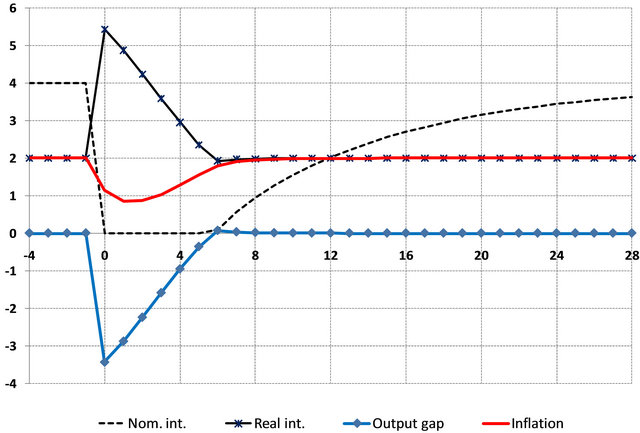
Figure 13. Impulse responses to a +7% risk shock with 0.9 persistence (and γ = 0.5) when the Central Bank tries to fully offset the effects of the shock (δ = 1), but cannot due to the 0-bound.
Impulse responses
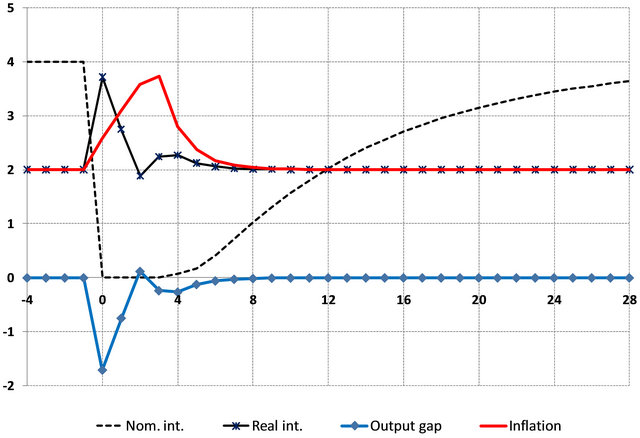
Figure 14. Impulse responses to the situation in Figure 13 along with a 4-quarter temporary increase in the inflation target from 2% to 4%.
flexible inflation expectations. Allowing inflation expectations to be determined as a weighted average of past inflation and the inflation target brings the exposition closer to rational expectations and allows for a discussion of costless disinflation. The inclusion of risk-premium shocks and the zero-bound on the policy rate allows for a discussion on the recent financial crisis and the ensuing liquidity trap. We also allow for deviations from the Taylor rule when setting monetary policy; this motivates a discussion regarding optimal policy response to demand shocks. These modifications to the textbook DADDAS model continue the trend of reducing the gap between undergraduate teaching of business fluctuations and the research frontier.
REFERENCES
- N. G. Mankiw, “Macroeconomics,” 7th Edition, Worth Publishers, London, 2010.
- J. Hicks, “Mr. Keynes and the ‘Classics’: A Suggested Interpretation,” Econometrica, Vol. 5, No. 2, 1937, pp. 147-159. doi:10.2307/1907242
- A. Abel, B. Bernanke and D. Croushore, “Macroeconomics,” 7th Edition, Prentice Hall, Upper Saddle River, 2010.
- C. I. Jones, “Macroeconomics,” 2nd Edition, W.W. Norton and Co., New York, 2010.
- F. S. Mishkin, “Macroeconomics: Policy and Practice,” Prentice Hall, Upper Saddle River, 2011.
- P. Bofinger, E. Mayer and T. Wollmershäuser, “The BMW Model: A New Framework for Teaching Monetary Economics,” Journal of Economic Education, Vol. 37, No. 1, 2006, pp. 98-117. doi:10.3200/JECE.37.1.98-117
- W. Carlin D. Soskice, “The 3-Equation New Keynesian Model—A Graphical Exposition,” Contributions to Macroeconomics, Vol. 5, No. 1, 2005, pp. 1-36.
- P. Kapinos, “A New Keynesian Workbook,” International Review of Economics Education, Vol. 9, No. 1, 2010, pp. 111-123.
- D. Romer, “Keynesian Macroeconomics without the LM Curve,” Journal of Economic Perspectives, Vol. 14, No. 2, 2000, pp. 149-169.
- A. Weerapana, “Intermediate Macroeconomics without the IS-LM Context,” Journal of Economic Education, Vol. 34, No. 33, 2003, pp. 241-262. doi:10.1080/00220480309595219
- C. Wiese, “A Simple Wicksellian Macroeconomic Model,” The B.E. Journal of Macroeconomics, Vol. 7, No. 1, 2007, Article 11.
- F. Smets and R. Wouters, “Shocks and Frictions in US Business Cycles: A Bayesian DSGE Approach,” American Economic Review, Vol. 97, No. 3, 2007, pp. 586-606. doi:10.1257/aer.97.3.586
- J. Gali, “Monetary Policy, Inflation, and the Business Cycle: An Introduction to the New Keynesian Framework,” Princeton University Press, Princeton, 2008.
- R. Clarida, J. Gali and M. Gertler, “The Science of Monetary Policy: A New Keynesian Perspective,” Journal of Economic Literature, Vol. 37, 1999, pp. 1661- 1707. doi:10.1257/jel.37.4.1661
- M. Kulish and C. Jones, “A Graphical Representation of an Estimated DSGE Model,” Dynare Working Papers Series #3, 2011.
- F. Kydland and E. C. Prescott, “Time to Build and Aggregate Fluctuations,” Econometrica, Vol. 50, No. 6, 1982, pp. 1345-1371. doi:10.2307/1913386
- C. E. Tovar, “DSGE Models and Central Banks,” Kiel Institute for the World Economy, Economics Discussion Papers 2008-30, 2008.
- B. S. Bernanke, M. Gertler and S. Gilchrist, “The Financial Accelerator in a Quantitative Business Cycle Framework,” In: J. B. Taylor and M. Woodford, Eds., Handbook of Macroeconomics, Elsevier Science, Amsterdam, 1999, pp. 1341-1393.
- S. Gilchrist, A. Ortiz and E. Zakrajsek, “Credit Risk and the Macroeconomy: Evidence from an Estimated DSGE Model,” Boston University, Boston, 2009.
- S. Alpanda, “Identifying the Role of Risk Shocks in the Business Cycle Using Stock Price Data,” Economic Inquiry, Vol. 51, No. 1, 2013, pp. 304-335. doi:10.1111/j.1465-7295.2011.00445.x
- P. Bofinger and S. Debes, “A Primer on Unconventional Monetary Policy,” CEPR Discussion PAPER: No. 7755, 2010.
- P. Kapinos, “Liquidity Trap in an Inflation-Targeting Framework: A Graphical Analysis,” International Review of Economics Education, Vol. 10, No. 2, 2011, pp. 91- 105.
- M. Woodford, “Interest and Prices,” Princeton University Press, Princeton, 2003.
- G. Calvo, “Staggered Prices in a Utility Maximizing Framework,” Journal of Monetary Economics, Vol. 12, No. 3, 1983, pp. 383-398. doi:10.1016/0304-3932(83)90060-0
- J. B. Taylor, “Aggregate Dynamics and Staggered Contracts,” Journal of Political Economy, Vol. 88, No. 1, 1980, pp. 1-23. doi:10.1086/260845
- J. Rotemberg, “Monopolistic Price Adjustment and Aggregate Output,” Review of Economic Studies, Vol. 49, No. 4, 1982, pp. 517-531. doi:10.2307/2297284
- O. J. Blanchard and C. M. Kahn, “The Solution of Linear Difference Models under Rational Expectations,” Econometrica, Vol. 48, No. 5, 1980, pp. 1305-1311. doi:10.2307/1912186
- J. B. Taylor, “Discretion versus Policy Rules in Practice,” Carnegie-Rochester Conference Series on Public Policy, Vol. 39, No. 1, 1993, pp. 195-214. doi:10.1016/0167-2231(93)90009-L
NOTES
*The views expressed in this paper are solely those of the authors. No responsibility for them should be attributed to the Bank of Canada.
#Corresponding author.
1Although early expositions of the IS-LM model were static, later versions have discussed dynamic adjustment of the economy to a long-run equilibrium identified with a full-employment level of output. This long-run adjustment is achieved through adjustment in the price level. This also renders the model consistent with long-run neutrality of money as prices increase proportional to the increase in the money supply in the long-run (Abel, Bernanke and Croushore [3]).
2DSGE models were initiated by the seminal work of Kydland and Prescott [16], which explored the role of productivity shocks in generating business cycles. Since then, these models have been expanded to include multiple shocks and various nominal and real rigidities, and have become commonplace tools in analyzing different sources of economic fluctuations, the impact of fiscal and monetary policy on macroeconomic variables, and in forecasting. See Tovar [17] for a recent discussion of these models and their use in central banks around the world.
3Weerapana [10], Bofinger and Debes [21], and Kapinos [22] also present pedagogical treatments of the liquidity trap, although they do not present the impulse responses.
4The Excel workbook accompanying this paper can be downloaded from our websites. Kapinos [8] also provides an accompanying Excel workbook. Our spreadsheet differs in that it allows for the analyses of risk shocks, the simultaneous effects of different shocks, or alternative forms of inflation expectations formation beyond adaptive expectations.
5The natural real interest rate is also known as the Wicksellian interest rate, and is the real interest rate that would prevail in the absence of nominal rigidities. Shocks that have an impact on the economy regardless of the presence of nominal rigidities (e.g. fiscal policy, productivity shocks etc.) would also alter the natural real interest rate (Woodford [23]) even in the short-run. We abstract from time-variation in the natural interest rate for simplicity, and focus on the long-run natural interest rate, which is a constant when the economy is hit only with temporary shocks.
6The assumption here that the risk-premium is equal to 0 at the steady-state is without loss of generality.
7The expectations term on the right-hand-side of the Phillips curve, which is past expectations of current inflation, follows Mankiw [1]. An alternative is to consider current expectations of future inflation (multiplied by a discount factor) instead. The latter can be motivated by the price-setting assumption in Calvo [24], where each period a fraction of randomly-selected firms are forced to keep their price the same as in the previous period. A similar expectations term also show up in models using the price-setting environment in Taylor [25] or Rotemberg [26]. For our purposes here, the distinction between these price-setting assumptions is not of major importance as long as the expected inflation term is determined as a combination of past inflation and target inflation. One way to motivate past inflation impacting current inflation in these other set-ups mentioned above (even in the presence of rational expectations) is to assume that there is partial inflation-indexation in price-setting (Smets and Wouters [12]).
8Note that this expectation equation is not strictly model-consistent, therefore not fully “rational”. For example, with γ = 0, agents always expect next period’s inflation rate to be at the target. In the presence of persistent shocks, rational agents would take into account that inflation may stay above the target level for a while. See Blanchard and Kahn [27] for imposing rational expectations to the solution of these models. As noted before, lagged inflation can still impact current inflation in the presence of rational expectations if there is inflation-indexation in price-setting.
9Alternatively, these deviations can be viewed as part of the Taylor rule when one acknowledges that the natural real interest rate is not a constant as modeled here, but is time-varying with demand-type shocks.
10Note that 1/α in front of the demand shock is to change the units of the demand shock from units of the output gap to units of the interest rate. In the benchmark calibration, α is set equal to 1 and hence the deviation from Taylor rule is of the same magnitude as the shocks.
11The specification in (1.6) already assumes that the Central Bank does not deviate from the Taylor rule when hit with cost-push shocks. If the loss function of the Central Bank solely depends on inflation and output gap volatility, there exist Taylor rule coefficients which are consistent with the optimal policy response to a cost-push shock, since the Taylor rule balances the inflation and output gap concerns of the Central Bank.
12In the DSGE literature with rational expectations, a similar result can be obtained by assuming that there is inflation indexation in price and wage-setting.
13If there are only demand shocks, then optimal policy can stabilize both inflation and output gap perfectly with strict inflation-targeting (this is also known as “divine coincidence”). In the presence of supply shocks, optimal policy balances the relative importance that the Central Bank places on these two macroeconomic indicators, which can be achieved via a Taylor rule.
13The credibility of the new inflation target is important since if the change in the inflation target is not credible, rational agents will still consider the previous higher inflation rate when forming expectations. In our exposition, we assume that the announced target changes by the Central Bank are credible. The presence of lagged inflation in inflation expectations may also be a proxy for the lack of credibility in the inflation target.