Wireless Engineering and Technology
Vol.4 No.3(2013), Article ID:34156,9 pages DOI:10.4236/wet.2013.43019
Suppression of Log-Normal Distributed Weather Clutter Observed by an S-Band Radar
![]()
1Department of Communications Engineering, National Defense Academy, Yokosuka, Japan; 2Department of Information Networks, Sendai National College of Technology, Sendai, Japan.
Email: sayama@nda.ac.jp
Copyright © 2013 Shuji Sayama, Seishiro Ishii. This is an open access article distributed under the Creative Commons Attribution License, which permits unrestricted use, distribution, and reproduction in any medium, provided the original work is properly cited.
Received May 1st, 2013; revised June 3rd, 2013; accepted June 17th, 2013
Keywords: CFAR; S-Band Radar; Weather Clutter; Log-Normal Distribution
ABSTRACT
We have observed weather clutter containing targets (ships) using an S-band radar with a frequency 3.05 GHz, a beamwidth 1.8˚, and a pulsewidth 0.5 μs. To investigate the weather clutter amplitude statistics, we introduce the Akaike Information Criterion (AIC). We have found that the weather clutter amplitudes obey the log-normal, Weibull, and log-Weibull distributions with the shape parameters of 0.308 to 0.470, 4.42 to 4.51, and 15.91 to 16.44, respectively, for small data within the beam width of an antenna. We have proposed the log-normal/CFAR circuit modified a Cell-Averaging (CA) LOG/CFAR circuit. It is found that weather clutter is suppressed with improvement of 51.58 dB by log-normal/CFAR. As a result, we have showed that weather clutter observed by S-band radar does not obey the Rayleigh distribution and our log-normal/CFAR circuit has an effect on suppression of clutter and detection of target, while conventional LOG/CFAR circuit does not. In addition, if our circuit can be realized, we will have an advantage economically.
1. Introduction
It is important for a marine radar to detect targets of ships. The radar displays azimuth and range to targets by polar coordinates on the round screen called PPI (Plan Position Indicator). But there is a noise called clutter besides targets in return signal. Such noise makes detection of targets difficult. To detect targets of ships in such clutter, anticlutter techniques have been improved [1].
Recently, many anticlutter techniques have been developed by using polarization, phase and so on. Because most of marine radars use only amplitude, such anticlutter techniques cannot be applied to these radars. But anticlutter technique by using amplitude has been hardly researched. Therefore, it is important to research anticlutter technique by using amplitude.
For example, a Constant False Alarm Rate (CFAR) circuit suppresses a false alarm probability low and constantly by using statistical characteristics of clutter amplitude. Here the false alarm probability is the probability that a clutter signal above a threshold level is misjudged as a target signal [2].
One of the CFAR circuit is the LOG/CFAR circuit making use of a logarithmic amplifier. When Rayleigh distributed clutter is passed through the LOG/CFAR circuit, this circuit keeps the variance of clutter output and the false alarm probability constant, that is, CFAR is obtained. But it has been found that clutter amplitude obeys non-Rayleigh distribution with advance of a high-resolution radar [3].
For example, we observed ground clutter which is the reflected waves from town and hill using an S-band radar having a frequency 3.05 GHz, a beam width 1.8˚, and a pulse width 1.0 μs. It was discovered that the ground clutter amplitudes obey the compound log-normal and compound log-Weibull distributions with the shape parameters of  0.217 to 0.429,
  0.028 to 0.410, and
  9.36 to 11.20,
  17.00 to 23.81, respectively, for small data within the beam width of an antenna [4].
Sea clutter which is the reflected waves from sea waves was measured using an X-band radar with a frequency 9.41 GHz, a beam width 1.0˚, and a pulse width . We found that the sea clutter amplitudes obey the log-normal, Weibull, log-Weibull, and generalized gamma distributions with the shape parameters of 0.467, 2.86 to 3.39, 9.37 to 10.76 and 2.52 to 4.18, respectively, for small data within the beam width of an antenna [5].
We observed weather clutter which is the reflected waves from rain and fog using an L-band long-range airroute surveillance radar (ARSR) having a frequency 1.3 GHz, a beamwidth 1.2˚, and a pulsewidth . It was discovered that the weather clutter amplitudes obey the Weibull distribution with the shape parameters of 2.07 for entire data and the Weibull, log-Weibull, and K-distributions with the shape parameters of 1.73 to 2.43, 10.60, and 5.13 to 50.93, respectively, for small data within the beam width of an antenna [6].
Moreover, sea ice clutter was measured using a millimeter wave radar with a frequency 34.86 GHz, a beamwidth 0.25˚, and a pulsewidth 30 ns. We found that the sea ice clutter amplitudes obey the log-Weibull distribution with the shape parameters of 2.97 for entire data and 2.69 to 3.15 for small data within the beam width of an antenna [7].
The Rayleigh distribution is identical to the Weibull distribution for  [8] and indicates the K-distribution in the region
  [9-12], so it is found that various clutter observed by various radars obey non-Rayleigh distribution.
If non-Rayleigh distributed clutter is passed through the LOG/CFAR circuit, then the false alarm probability is not kept constant by a wrong threshold level. And then targets have been embedded in clutter which cannot be suppressed or have been erased on a PPI screen. Therefore, it is necessary to devise a new CFAR circuit for suppression of non-Rayleigh distributed clutter.
In the following, we have observed weather clutter data containing targets of ships using an S-band radar with a frequency 3.05 GHz, a beamwidth 1.8˚, and a pulsewidth 0.5 μs. We investigate the weather clutter amplitudes by using the Akaike Information Criterion (AIC) [13] and four probability distribution models. It is found that weather clutter amplitudes obey non-Rayleigh distribution. Therefore, we propose a new log-normal CFAR circuit modified a Cell-Averaging (CA) LOG/CFAR circuit. We apply this circuit and conventional LOG/CFAR circuit to the observed data, it is found that this circuit has an effect on suppression of clutter and detection of target, while conventional LOG/CFAR circuit does not. In addition, if our circuit can be realized, we will have an advantage economically.
The paper is organized as follows: In Section 2, we indicate radar system and describe weather clutter observed by this system. Explanations of four probability distribution models and AIC and result of distribution estimation are given in Section 3. We propose the log-normal/CFAR circuit modified a CA LOG/CFAR circuit and apply this circuit to weather clutter in Section 4.
2. Observations of Weather Clutter by an S-Band Radar
As mentioned in Section 1, various clutter make detection of targets difficult in a radar. The most considerable clutter is weather clutter in an S-band marine radar. Because X-band radars installed together in many ships cannot be used in rain. Therefore, we observed weather clutter data containing targets of ships using an S-band radar. Here, we explain the radar used for observation and the radar system used for record of data. And we illustrate the observed data.
2.1. Radar System
S-band radar used for observation is installed at the National Defense Academy in Yokosuka-City. The S-band radar characteristics are given in Table 1.
The radar system block diagram is shown in Figure 1. The antenna rotation signal (AZP) and the head marker (AZR) were always sent from the radar to the azimuth control unit. The sampling start signal was sent from the azimuth control unit to the personal computer (IBM PC) through the PS/2 terminal or the USB terminal. Then, the video signal from the radar was digitized in 8-bit (256 levels) by the A/D converter. The 8-bit digitized data were transferred to the hard disk drive through the bus controller and were displayed in the monitor at the same time. The region of the observed data recorded was set up by the azimuth control unit. According to this setup, the azimuth direction and the radial direction were controlled by the trigger signal from the radar. The sampling rate of A/D convert was set by the personal computer and was 20 MHz in this time.

Table 1. S-band radar parameters.

Figure 1. Radar system block diagram.
2.2. Observed Data
The observed data is shown in Figure 2. We observed it at 18:46 December 11, 2009. The observation was made in area including the Uraga Suido Traffic Route off Cape Futtu, Chiba Prefecture. On that day, it was rain. The precipitation was 3.5 mm/h. The wind was in the north, the wind velocity was 7 m/s. Because it was foggy, when the ships entered the Uraga Suido Traffic Route, they gave the fog alarms. The observed data was from 25.2˚ to 47.7˚ in the azimuth direction and from 3.91 km to 5.81 km in the radial direction. The observed data was a region of 256 range sweeps in azimuth and 256 range bins in radial interval. The data points totaled 65,536. The reflection amplitude at each point was quantized to 256 levels. The observed data is represented in gray scale as 256 gradation from the black of amplitude 0 to the white of 255.
Weather clutter from rain and fog looks white in the figure. Two targets surrounded by circles of white broken line are a passenger ship SARUBIA MARU with a ship length 121 m in upper left and a cargo ship HOEGH AMERICA with a ship length 200 m in lower right. The information about ship names and lengths were gotten from the AIS (Automatic Identification System). In the figure, the vertical lines are radar interference with other radars having the same frequency. Many ships pass through the Uraga Suido Traffic Route while they operate radars having the same frequency. Therefore, such a radar interference occurs.
3. Distribution Estimation of Weather Clutter
To estimate a distribution model obeying clutter amplitude, we apply some models to observed data and compare “goodness” of models. In this paper, we use four probability distribution models, the log-normal, Weibull, log-Weibull, and K-distributions, and introduce the Akaike Information Criterion (AIC). Here, we explain the probability density functions and the properties of these four models and summarize the AIC.
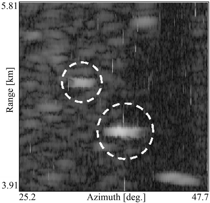
Figure 2. Observed data.
3.1. Distribution Estimation Models
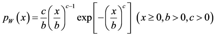
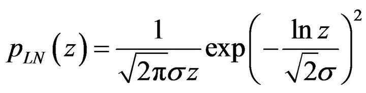
The log-normal distribution is written as follows:
 (1)
(1)
Here  is the amplitude of the return signals,
  is an average of
  (a scale parameter) and
  is the standard deviation of
  (a shape parameter). The character of this distribution is its long tail. Recently, to develop a high-resolution radar, return signals accompany many spikes. It has been observed that the clutter amplitude has a longer tail [8].
The Weibull distribution was proposed by Prof. Walodi Weibull at the Swedish Royal Institute of Technology in 1939 [14]. This distribution is written as follows:
 (2)
(2)
Here  is a scale parameter and
  is a shape parameter. It is important that the Weibull distribution includes the exponential and Rayleigh distributions. That is, for
  and 2.0 in Equation (2), the Weibull distribution is identical to the exponential and Rayleigh distributions, respectively [8].
We proposed a new log-weibull distribution as the probability distribution model for clutter [4,15]. The logWeibull distribution is written as follows:
 (3)
(3)
Here  is a scale parameter and
  is a shape parameter. The log-Weibull distribution has the advantage of both the log-normal and Weibull distributions. That is, the log-Weibull distribution has a long tail and is flexible in its shape.
The K-distribution was proposed by E. Jakeman and P. N. Pusey in 1976 [9]. This distribution is written as follows:
 (4)
(4)
Here  is a scale parameter and
  is a shape parameter.
  is the gamma function and
  is the
  th modified Bessel function.
  has been found to lie in the region
 , indicating Rayleigh distributed clutter. The smaller the value of
  becomes, the longer the tail of the K-distribution becomes and the larger the gap between the Rayleigh and K-distributions becomes [9-12]. The K-distribution includes the modified Bessel function. Therefore, the K-distribution is more difficult than the other three distributions in its calculation.
3.2. The Akaike Information Criterion (AIC)
Now we assume that the  numbers of the independent values
  are observed. We consider applying a model
  to these observed data (
 are parameters of the probability density function of this model). The logarithmic likelihood
  of this model is defined as
 . (5)
. (5)
We obtain  (the maximum likelihood estimation) which gives the largest
  and select the
  (the maximum likelihood model). Considering some given probability distribution models, we select the model which gives the largest logarithmic likelihood, and we obtain the nearest model to the true probability distribution. The expectation for data
  of the average logarithmic likelihood of the maximum likelihood model corresponds to the expectation average logarithmic likelihood. The maximum likelihood is considered as an estimation of the expectation average logarithmic likelihood. On detailed investigation, we find the bias that the maximum likelihood tends to be larger than the true expectation average logarithmic likelihood. We investigate the relationship between the extent of the bias and the number of parameters included in the model. It is found that
 (6)
(6)
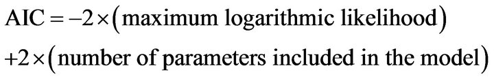
is approximately an unbiased estimation of the expectation average logarithmic likelihood. According to historical circumstances, Equation (6) multiplied by –2 is called AIC [13]. That is,
 (7)
(7)
The AIC is not the Kullback-Leibler entropy [16] but the expectation average logarithmic likelihood estimation. The AIC does not depend on each value of data and is determined by the true probability distribution of data, the number of data, and the model. Therefore, the value of the AIC itself is not significance, the differences in the values of the AIC are important. The significant differences are larger than unity from the relationship between the AIC and the entropy. The model which yields the smallest AIC (MAIC; minimum AIC estimation) is regarded as the best one [17].
3.3. Result of Distribution Estimation
In general, return signals have strong correlation and the same properties within the beam width of an antenna. Thus we divide the observed data into small data within the horizontal beam width of an antenna 1.8˚. We estimate each small data by using the AIC and four probability distribution models.
Here, a range sweep number (0 - 255) is assigned to 256 points in azimuth direction. From the relation between the horizontal beam width of an antenna and the range sweep number, the horizontal beam width of an antenna 1.8˚ is correspond to the range sweep number 20 points. The observed data in Figure 2 is divided into every 20 points like strips. The number of small data is 12 and the number of its data points is 5120.
We summarize the parameters and the values of the AIC for different range sweep numbers in Table 2. The smallest AIC (MAIC) are indicated by underline. The numbers of the MAIC of the log-normal, Weibull, logWeibull, and K-distributions are 8, 2, 2, and 0, respecttively, from 12 small data within the beam width of an antenna. The log-normal distribution is best fit to data for 8 small data more than half of the entire data. Moreover, the log-normal distribution is best fit to data for 5 small data of 6 small data containing targets (range sweep 60 - 179).
In Table 2, we have found that the weather clutter amplitudes observed by an S-band radar obey the lognormal, Weibull, and log-Weibull distributions with the shape parameters of 0.308 to 0.470, 4.42 to 4.51, and 15.91 to 16.44, respectively, for small data within the beam width of an antenna. If clutter obeyed the Rayleigh distribution, clutter amplitude should obey the Weibull distribution for . But, there is no such small data. It is found that all small data obey non-Rayleigh distribution.
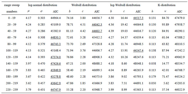
Table 2. Result of distribution estimation for different range sweep numbers.
Examples of small data obeying the log-normal, Weibull, and log-Weibull distributions are illustrated in Figures 3-5, respectively. In any case, the distribution estimation models are best fit to data.
4. Log-Normal/CFAR Circuit Modified a Cell-Averaging LOG/CFAR Circuit
It has been discovered that weather clutter observed by an S-band radar obeys non-Rayleigh distribution. It is necessary to devise a new CFAR circuit in order to suppress such clutter and detect targets. If we can realize the new CFAR circuit by modifying the LOG/CFAR circuit which had been already put to practical use, we will have an advantage economically. It has been found that the log-normal distribution is best fit to data for many small data containing targets in Section 3.3. Therefore, we propose a new log-normal CFAR circuit modified a CellAveraging (CA) LOG/CFAR circuit.
The log-normal CFAR circuit modified a CA LOG/ CFAR circuit is shown in Figure 6. This circuit can be realized by only adding a circuit calculating a meansquared value to a conventional CA LOG/CFAR circuit. Here, it is logically explained how this circuit maintains CFAR for log-normal distributed clutter.
4.1. The CFAR Maintenance in Log-Normal Distributed Clutter
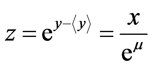
In Figure 6, if the clutter signal  obeying the lognormal distribution in Equation (1) is passed through an idealized logarithmic amplifier, the output signal
  is
is
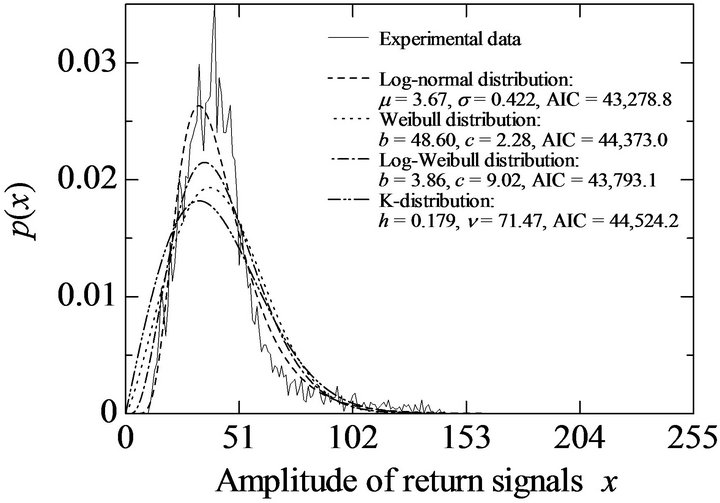
Figure 3. Log-normal distribution is best fit to data in range sweep 180 - 199.
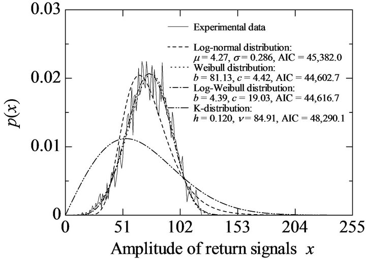
Figure 4. Weibull distribution is best fit to data in range sweep 40 - 59.
represented by
 (8)
(8)
 is put in a delay line, the mean signal level of
  is calculated,
  is
is
 (9)
(9)
Subtracting  from y, the output signal z passed through an antilogarithmic amplifier is represented by
 (10)
(10)
And Equation (1) is transformed into the probability
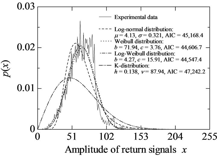
Figure 5. Log-Weibull distribution is best fit to data in range sweep 100 - 119.
density function of  by using Equation (10).
  is given by
 (11)
(11)
When a threshold level  is set to the signal
  obeying the distribution represented by Equation (11), since the signal of
 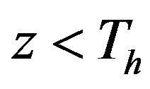 becomes
  by a comparator, the false alarm probability
  is given by
 (12)
(12)
Here, erf( ) is the error function.  is independent of
  and depends on
 . That is,
  changes by the value of
  and is not constant. CFAR is not maintained.
But, in Equation (12), if the value of  has been already obtained,
  can be set in order to keep
  constant according to the value of
 . CFAR can be maintained. To obtain
 , by using a new additional circuit calculating a mean-squared value, the meansquared signal level
  becomes
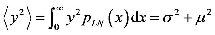 (13)
(13)
Now,  is squared and subtracted from
 . The variance of
  is given by
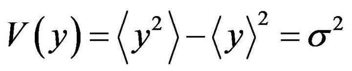 (14)
(14)

Figure 6. Log-normal/CFAR circuit modified a Cell-Averaging (CA) LOG/CFAR circuit.
 is independent of
  and depends only on
 . That is,
  can be determined by calculating
 . Therefore, if
  can be calculated besides
  calculated by a CA LOG/CFAR circuit,
  can be calculated from
 . If the comparator decides whether there is target or not by
  set according to
 ,
,  is kept constant. That is, it is possible to maintain CFAR for the log-normal distributed clutter.
 for obtaining aimed
  is determined by substituting
  calculated from Equation (14) into Equation (12). But, Equation (12) corresponds to the case of a sample number
  in Figure 6. When the CA LOG/CFAR circuit is used practically,
  is finite. Moreover,
  becomes a comparatively small value, because a radar is operated almost in real time. It is impossible to use Equation (12) representing
  for
for . Therefore, random numbers obeying the lognormal distribution were generated by the multiplicative congruential method on a computer. The random numbers were passed through the CA LOG/CFAR circuit in Figure 6. On every values of
 , we set
  to the output
 .
.  were calculated as the probability of
  exceeding
 .
.  were calculated at intervals of 0.001, and
  were calculated down to two decimal places. Each of the number of generated random numbers were 100,000,000.
Example is shown in Figure 7. The random numbers obeying the log-normal distribution with  were generated. The relation between
  and
and  were calculated for
 , 4, 8, 16, 32, 64, and 128. For example,
  is assumed to be
 .
.  is determined as an intersection in curve and broken line.
  is determined 3.47, 3.12, 2.94, 2.85, 2.81, 2.79, and 2.78, respectively.
4.2. Log-Normal/CFAR Processing Results
We applied the log-normal/CFAR circuit modified a CA
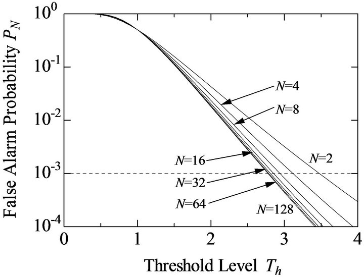
Figure 7. Threshold level  versus false alarm probability
 .
.
LOG/CFAR circuit to the observed data in Figure 2. First, to evaluate the log-normal/CFAR circuit quantitatively, we introduce the target-to-clutter ratio. The targetto-clutter ratio  is defined as
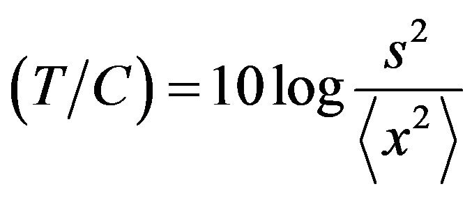 (15)
(15)
Here, s and x are the signals of target and clutter, respectively [18].
When the observed data was actually processed by this circuit for the sample number 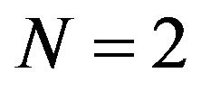 and 4, two and four consecutive signals of same values were occasionally put in both sides of the test cell on the delay line. The variance became
 , that is,
 . The threshold level
  could not be calculated. For
  and 16, the values of
  occasionally became extremely big or small values which were completely different from the results of distribution estimation in Section 3.3. (For example, the maximum and minimum values of
  were 0.008 and 0.855 for
 , respectively.) Therefore, for
 , 4, 8, and 16, it is of no practical use.
Next, for , 64, and 128, since the number of data is 65,536, the false alarm probability
  is set to
 ,
,  , and
, and . We calculate the target-to-clutter ratio
  from Equation (15) and summarize the ratio
  in Table 3. The unit is dB. In Table 3,
  cannot be calculated for
 and
and  and
and ,
,  , because clutter can be suppressed but the targets cannot be detected by lognormal/CFAR processing.
  of the observed data is 7.85 dB. Therefore
  is improved on all lognormal/CFAR processing except them. A maximum of
  is 59.43 dB for
 ,
,  Thus we obtain a maximum improvement of 51.58 dB.
The samples of log-normal/CFAR processing image are shown in Figures 8 and 9. These are processed for ,
,  and
and , respectively. Here, as white and black in Figure 2 are reversed, the processed images are represented in gray scale as 256 gradation from the white of amplitude 0 to the black of 255. To make easily to see, a maximum of signal after processing is normalized to 255. Circles of black broken line correspond to circles of white broken line in Figure 2. In Figure 8, the targets are completely detected. The meas-

Table 3.  of log-normal/CFAR processed results.
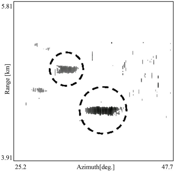
Figure 8. Log-normal/CFAR processed image (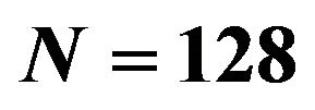 ,
, ).
).
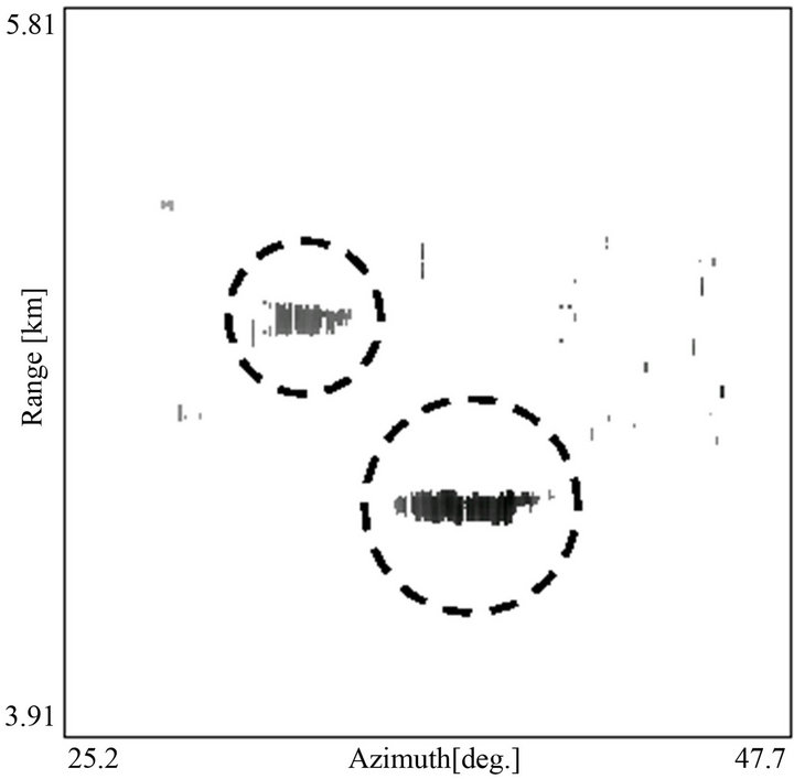
Figure 9. Log-normal/CFAR processed image ( ,
, ).
).
urement value of false alarm probability  is 1.3 × 10⁻². It is almost equal to the theory value. While, in Figure 9, part of targets are disappeared and targets are not completely detected. the measurement value of
  is 4.8 × 10⁻³. It is larger than the theory value. Because, calculating threshold levels on a computer, we did not consider the correlation between radar signals. In Figures 8 and 9, the vertical lines representing radar interference are not disappeared. Because the radar interference is artificial signal and does not obey the log-normal distribution.
To compare with the log-normal/CFAR processed image, the conventional LOG/CFAR processed image is shown in Figure 10. This is processed for ,
, . In Figure 10, white and black are reversed as in Figures 8 and 9. Clutter is suppressed but the target of SARUBIA MARU in upper left is disappeared and cannot be detected. Though weather clutter does not obey the Rayleigh distribution, it is processed by the LOG/ CFAR circuit. Therefore, the threshold level
  is too high, a target signal cannot exceed
  and target is disappeared.
5. Conclusions
We observed weather clutter data containing targets of ships using an S-band radar with a frequency 3.05GHz, a beamwidth 1.8˚, and a pulsewidth . We investigated the weather clutter amplitudes by using the AIC and four probability distribution models. It is found that weather clutter amplitudes obey the log-normal, Weibull, and log-Weibull distributions with the shape parameters of 0.308 to 0.470, 4.42 to 4.51, and 15.91 to 16.44, respectively, for small data within the beam width of an antenna, and many small data containing targets obey the log-normal distribution. Therefore, we propose a new log-normal CFAR circuit modified a CA LOG/CFAR circuit. We apply this circuit to the real observed data, it is found that weather clutter is suppressed with a maximum improvement of target-to-clutter ratio 51.58 dB.
In the future, we will observe sea and ground clutter, and apply this circuit to such clutter. Then we will examine whether this circuit has an effect on suppression of such clutter or not. We will plan to develop the circuit
Figure 10. LOG/CFAR processed image (N = 128, PN = 10−2).
which can suppress two or three kinds of clutter at the same time.
REFERENCES
- D. K. Barton, “Radar Clutter,” Artech House, Dedham, 1975.
- J. Croney, “Clutter on Radar Displays,” Wireless Engineering, Vol. 33, 1956, pp. 83-96.
- M. Sekine, “Radar Signal Processing Techniques,” The Institute of Electronics, Information and Communication Engineers, Tokyo, Japan, 1991 (in Japanese).
- S. Sayama and S. Ishii, “Amplitude Statistics of Ground Clutter from Town and Hill Observed by S-band Radar,” IEEJ Transactions Fundamentals and Materials, Vol. 131, No. 11, 2011, pp. 916-923 (in Japanese). doi:10.1541/ieejfms.131.916
- S. Sayama and S. Ishii, “Amplitude Statistics of Sea Clutter by MDL Principle,” IEEJ Transactions Fundamentals and Materials, Vol. 132, No. 10, 2012, pp. 886-892 (in Japanese). doi:10.1541/ieejfms.132.886
- S. Sayama, S. Ishii and M. Sekine, “Amplitude Statistics of Weather Clutter Observed by L-Band Radar,” IEEJ Transactions Fundamentals and Materials, Vol. 126, No. 6, 2006, pp. 438-442. doi:10.1541/ieejfms.126.438
- S. Sayama and M. Sekine, “Observations and Suppression of Sea Ice Clutter by Means of Millimeter Wave Radar,” IEICE Transactions on Communications (Japanese Edition), Vol. J85-B, No. 7, 2002, pp. 1104-1111 (in Japanese).
- M. Sekine and Y. Mao, “Weibull Radar Clutter,” Peter Peregrinus Ltd., London, 1990. doi:10.1049/PBRA003E
- E. Jakeman and P. N. Pusey, “A Model for Non-Rayleigh Sea Echo,” IEEE Transactions on Antennas and Propagation, Vol. AP-24, No. 6, 1976, pp. 806-814. doi:10.1109/TAP.1976.1141451
- J. K. Jao, “Amplitude Distribution of Composite Terrain Radar Clutter and the K-Distribution,” IEEE Transactions on Antennas and Propagation, Vol. AP-32, No. 10, 1984, pp. 1049-1062. doi:10.1109/TAP.1984.1143200
- S. Watts, “Radar Detection Prediction in Sea Clutter Using the Compound K-Distribution Model,” IEE Proceedings, Vol. 132, No. 7, 1985, pp. 613-620. doi:10.1049/ip-f-1.1985.0115
- S. Watts, “Radar Detection Prediction in K-Distributed Sea Clutter and Thermal Noise,” IEEE Transactions on Aerospace and Electronic Systems, Vol. AES-23, No. 1, 1987, pp. 40-45. doi:10.1109/TAES.1987.313334
- H. Akaike, “Information Theory and an Extension of the Maximum Likelihood Principle,” In: B. N. Petrov and F. Csaki, Eds., 2nd International Symposium on Information Theory, Akademiai Kiado, 1973, pp. 267-281.
- W. Weibull, “A Statistical Theory of Strength of Materials,” IVB-Handl., 1939, No. 151.
- M. Sekine, T. Musha, Y. Tomita, T. Hagisawa, T. Irabu and E. Kiuchi, “Log-Weibull Distributed Sea Clutter,” IEE Proceedings, Vol. 127, No. 3, 1980, pp. 225-228. doi:10.1049/ip-f-1.1980.0033
- S. Kullback and R. A. Leibler, “On Information and Sufficiency,” Annals of Mathematical Statistics, Vol. 22, No. 1, 1953, pp. 79-86. doi:10.1214/aoms/1177729694
- Y. Sakamoto, M. Ishiguro and G. Kitagawa, “Information Statistics,” Kyoritsu Shuppan Co., Ltd., Tokyo, 1983 (in Japanese).
- M. Sekine and N. Oura, “Introduction to Electrical and Electronic Measurements,” Shoko-do, Tokyo, 2006 (in Japanese).