Journal of Environmental Protection
Vol.08 No.10(2017), Article ID:79100,20 pages
10.4236/jep.2017.810066
Energy-Saving Scheduling in a Flexible Flow Shop Using a Hybrid Genetic Algorithm
Rong-Hwa Huang1, Shun-Chi Yu2, Po-Han Chen1
1Department of Business Administration, Fu Jen Catholic University, Taiwan
2Department of Tourism and Hospitality, China University of Science and Technology, Taiwan

Copyright © 2017 by authors and Scientific Research Publishing Inc.
This work is licensed under the Creative Commons Attribution International License (CC BY 4.0).
http://creativecommons.org/licenses/by/4.0/


Received: August 11, 2017; Accepted: September 12, 2017; Published: September 15, 2017
ABSTRACT
Many researches discussing reduced energy consumption for environmental protection focus on machine efficiency or process redesign. To optimize the machine operation time can also save the energy, and these researches have received great interests in recent years. This study considers three different states of machines, among processing there are two different speeds, to solve the problem of minimizing energy costs under time-of-use tariff with no tardy jobs in flexible flow shop. This problem is basically NP-hard, we proposed a hybrid genetic algorithm (GA) to solve problems in reasonable timeliness. The result shows that to optimize different states of machines under time-of use tariff can reduce energy costs significantly in on-time delivery.
Keywords:
Flexible Flow Shops, Energy-Saving Genetic Algorithm, Energy Consumption Cost, Non-Tardy, Genetic Algorithms

1. Introduction
Goldratt and Cox [1] posit that goal achievement by a goal-oriented system is limited by at least one constraint. The limitation of electricity affects the energy in Taiwan. Good energy-saving production systems have become important issue during peak time. In practical production, energy saving is essential for enhancing production activity and maximizing the effectiveness of processes on machines. The electricity consumption of industries exceeds half of global consumption and affects the operating efficiency in practical situations.
A flexible flow shop (FFS) scheduling problem provides multiple identical parallel machines at each station for increasing capacity and reducing costs. Flow shop processing involves constant sequences of initial, standard, steady, and nonpermutable production, such as that of steel, optoelectronics, and metal, which are common in real-world situations [2] [3] . To offer widely application, Linn and Zhang [4] indicated that FFS scheduling applies to traditional flow shop situations. The attempted problem is excellently solved. However, the energy consumption of machines affects the efficiency and quality of production; for instance, increased on-peak electricity consumption of machines causes an increase in temperature, wearing of parts, and improper manual operation. The time-of-use (TOU) tariff is a common used for adjusting peak power consumption worldwide. Generally, the billing period is divided into on-peak hours, mid-peak hours, and off-peak hours. The electricity costs during the on-peak period are the highest, whereas those during the off-peak period are the lowest. Moreover, machines can be switched to operation, standby, and shutdown modes for preventing unnecessary energy wastage.
As for trade-off of energy saving method, Ribas et al. [5] demonstrated that enterprises added machines to certain stages, thus enhanced production efficiency and customer satisfaction. An energy-efficient mathematical model for solving FFS scheduling problems and multiobjective optimization to minimize the makespan and total energy consumption [6] . The experimental results showed that the relationship between the makespan and energy consumption may be conflicting. A proposed energy-saving decision is useful for minimizing energy consumption. To minimize trade-off of earliness and tardiness in a practical production environment, Huang et al. [7] developed a farness particle swarm optimization (FPSO) algorithm for solving reentrant two-stage multiprocessor flow shop scheduling problems.
As for energy-saving issues, because of scarce resources, increasing attention has been focused on developing practical production techniques for clean technologies and protecting the environment [8] . Decreasing emission of CO2 attracts more attentions. Zhang et al. [9] developed a time-indexed integer programming formulation for solving manufacturing schedules that minimize electricity cost and the carbon footprint under TOU tariffs without compromising production throughput. The proposed method used a flow shop with eight process steps that were operated on a typical summer day for an energy-saving test. Results indicated that shifting electricity usage from on-peak hours to mid-peak hours or off-peak hours reduces electricity costs; however, it may increase CO2 emissions in regions where the grid base load is met with electricity from coal-fired power plants. The tradeoff between minimizing electricity cost and reducing CO2 emissions was shown using a Pareto frontier. Setlhaolo [10] demonstrated that using residential demand response along with a mixed integer nonlinear optimization model under a TOU electricity tariff can solve the scheduling problem of typical home appliances as well as minimize electricity costs and facilitate earning relevant incentives [11] . An analysis revealed that households can alter their electricity consumption in response to varying prices and incentives; thus, a consumer may reduce electricity costs by more than 25%. Different values of the weighting factor (α) provide varying costs. According to the α values and their preferences, consumers can choose their electricity costs. FFS scheduling can save energy and lower manufacturing costs by clean technologies, environmental policy, reducing the completion time and inventory in industrial environments.
Energy-saving models are created for important issues, Mouzon and Yildirim [12] developed operational methods for minimizing the energy consumption of manufacturing equipment and total completion time. The energy used in processes can be saved by turning off nonbottleneck (i.e., underutilized) machines or equipment when they are idle for a certain period of time. In particular, an analysis indicated that the proposed dispatching methods are effective in reducing the energy consumption of underutilized manufacturing equipment. Therefore, a production manager has a set of nondominated solutions (i.e., a set of efficient solutions) that he or she can use for determining the most efficient production sequence; moreover, they minimize the total energy consumption while optimizing the total completion time. Fang et al. [13] developed a new mathematical programming model for flow shop scheduling problems to minimize the peak power load, energy consumption, and associated carbon footprint along with the cycle time. In a flow shop with two machines producing various parts, the operation speed was considered an independent variable, which can be changed to affect the peak load and energy consumption. The results demonstrated that the proposed approach enables determining near-optimal schedules for achieving energy-saving goals. Tibi and Arman [14] developed a mathematical linear programming model to optimize the decision-making for managing a cogeneration facility as a potential clean-development mechanism project in a hospital in Palestine. The model optimized the cost of energy and the cost of installation of a small cogeneration plant under constraints on electricity-and-heat supply and demand balances. The results proved the efficiency of the proposed method. He et al. [15] demonstrated that the environmental load resulting from the energy consumption of machine tool systems is broadly recognized. Improving scheduling saves energy, facilitates efficient use of machine tools, and reduces energy consumption by idle equipment. One proposed energy-saving optimization method involves machine tool selection and a series of machine operations for flexible job shops. The method was designed to reduce the energy consumption of machine operations, and the scheduling was aimed at reducing the unused power consumption of machine tools. The current study investigated how to develop and use clean technologies like non-tardy procedures for scheduling the use of parallel machines to maintain practical production for environmental protection.
To prevent tardiness and ensure effective operation of production equipment, companies create effective and efficient production environments that maximize corporate benefits from production activities. Bruzzone et al. [16] developed energy-aware scheduling of manufacturing processes by using advanced planning and scheduling, a mathematical model for optimally planning energy saving for a given schedule. The new approach relies on the MIP model, where the reference schedule is modified to account for energy consumption without changing the jobs’ assignments and sequencing provided by the reference schedule. The results demonstrated that a commercial MIP solver and an original MIP heuristic are applicable in practical production.
Enumeration and heuristic methods have been applied for energy saving in previous studies [10] . Integer programming, branch and bound programming, and MIP are the most widely used enumeration methods that can provide appropriate solutions. However, high computational times limit the applicability of enumeration methods to small-scale problems [17] . Thus, heuristics such as the genetic algorithm, simulated annealing algorithm, and ant colony optimization algorithm are commonly used for solving energy-saving problems. Lian [18] obtained the average relative error rates of −28.20% and 60.25% for a combined local and global PSO algorithm against PSO and genetic algorithms, respectively. Zhang et al. [19] presented an I-ATTPSO algorithm with an average effectiveness improvement rate of −14% in small-scale problems and 55% in large-scale problems. Liu et al. [20] obtained an average relative error rate of 0.65% for the PSO-EDA_PI algorithm against other algorithms. Zhao et al. [21] found the average relative error rate of their proposed logistic dynamic PSO algorithm against other algorithms to be approximately 1.19% - 2.39%.
In many industrialized countries, manufacturing industries pay stratified electricity charges depending on the time of the day (i.e., on-peak, mid-peak, and off-peak hours) [22] . China saves energy concerning the impact of internal industrial configuration in terms of size and ownership structure on aggregate energy intensity [23] . Besides, Germany property owners can deduce where they should ideally invest in order to optimize the energy efficiency of their building stock sustainably [24] . By contrast, the emerging smart grid concept may demand that industries pay real-time hourly electricity costs for the efficient usage of energy. To enable decision makers to apply feasible solutions for resolving unrelated parallel machine scheduling problems, Moon et al. [25] developed an energy-efficient method by using the weighted sum objective of production scheduling and electricity usage. Reliability models using a hybrid genetic algorithm along with their blank job insertion algorithm consider the energy cost aspect of the problem with the objective function of optimizing the weighted sum of two criteria: the minimization of the production makespan and the minimization of time-dependent electricity costs. The results demonstrated its performance in simulation experiments in practical production.
Energy-saving method relates to fixed costs. Shrouf et al. [26] posited that rising energy costs associated with increased production costs at manufacturing facilities encouraged decision makers to tackle this problem in different ways. One crucial step in this trend is to reduce the energy consumption costs of production systems. Considering variable energy prices in a single day, the authors proposed a mathematical model for minimizing energy consumption costs for single machine production scheduling during production processes. The job processing time consists of the starting time, idle time, and times when the machine must be shut down, turned on, and turned off. The proposed mathematical model enables the operation manager to implement the least expensive production scheduling during a production shift. To obtain feasible solutions by using a genetic algorithm, this study also determined whether the heuristic solution provides the minimum cost and optimal schedule for minimizing energy costs. In addition, an analytical solution was applied to generate the optimal solution. Moreover, analytical solutions and heuristic solutions were compared, and the heuristic solution is considered preferable for larger problems. The results indicate that significant reductions in energy costs can be achieved by avoiding high-energy price periods. The results have a positive environmental effect by reducing energy consumption during peak periods, thereby increasing the possibility of reducing CO2 emissions from power generator sites. Although a genetic algorithm can efficiently solve energy-saving problems and prevent entrapment at a local optimum, the current study improves the solving process for enhancing performance in practical production and environmental protection.
By applying the nontardy constraint to practical production, the current study attempted to minimize makespan costs. A Cmax minimization genetic algorithm (CGA) and energy minimization genetic algorithm (EGA) are proposed for use in the first stage of solving two-stage multiprocessor flow shop scheduling problems and minimizing makespan costs. Furthermore, an adjusted Cmax minimization genetic algorithm (ACGA) and adjusted energy minimization genetic algorithm (AEGA) used in the second stage were compared for obtaining superior solutions and aiding enterprises in increasing profits and lowering overhead costs. The current study compared the proposed solution with two reported solutions that yielded comparable improvements.
The remainder of the paper is organized as follows: In Section 2, the FFS is formulated. In Section 3, the basic algorithms are introduced briefly. Then, the framework of energy-saving genetic algorithm for solving the FFS is proposed in Section 4. The influence of parameter setting is investigated based on design of experiment testing in Section 4, and computational results and comparisons are provided as well. Finally, we end the paper with some conclusions in Section 5.
2. Problem Definition
According to notation rule of Pinedo [27] , the current study formulates the problem as . represents k-stage flexible flow shop scheduling environment. means different electricity bill in each period. denotes three conditions of operation: stand-by, or shut-down of machines, and re-operation of machines also consumes power. demonstrates all operations of non-tardy jobs must complete before completion dates in order to minimize electricity costs. Figure 1 demonstrates the Gantt

Figure 1. State of machine process.
chart of the attempted problem.
The FFS problem provides multiple identical parallel machines at each station for increasing capacity and reducing costs in practical production. One machine at every station can be selected for each job and the process begins from the first station. After the final job is completed in the second stage, all jobs are completed.
The scope and constraints of this study are demonstrated as follows:
1) Number of jobs, machines and stages are known.
2) Processing time of each job on each machine is known and constant.
3) Each machine in each stage can only process one job simultaneously.
4) The sequence through which jobs pass through machines may differ with the sequence of machine receiving job.
5) Jobs cannot be preempted.
6) There is no permutation, or machine breakdown.
7) The job ready time is 0.
8) Machines can switch into operation, stand-by, and shut-down.
2.1. Notation
= total period set, all jobs in this study
= total parallel machines at stage i, all machines in this study
= due date set, all jobs completed dates in this study
= job set, all jobs waiting for scheduling in this study
= stage set, all stages in this study
= the maximal completion time of all jobs
= the due date of job
= the completion time of job processed in the m-th machine at the k-th stage
= the starting time of job processed in the m-th machine at the k-th stage
= the processing time of job processed in the m-th machine at the k-th stage
= the turn-on energy consumption of all machines at t-th time
= the stand-by energy consumption of all machines at t-th time
= the working energy consumption of all machines at t-th time
= the working energy consumption in the m-th machine at the k-th stage
= the stand-by energy consumption in the m-th machine at the k-th stage
= the working energy consumption of job processed in the m-th machine at the k-th stage
= the electricity bill of different time period
= indicator of whether job is scheduled at the k-th stage in m-th machine at t-th time ( = (0, 1); if = 1, job is processed at the k-th stage in m-th machine at t-th time; otherwise = 0)
= indicator of whether job is assigned at the k-th stage in m-th machine at t-th time ( = (0, 1); if = 0, job is processed at the k-th stage in m-th machine at t-th time; otherwise = 1)
= indicator of whether at the k-th stage the m-th machine turned on at t-th time ( = (0, 1); if = 1, the m-th machine was turned on at t-th time; otherwise = 0)
= indicator of whether at the k-th stage the m-th machine turned off at t-th time ( = (0, 1); if = 0, the m-th machine was turned off at t-th time; otherwise = 1)
2.2. Mathematical Model
1) Objective function
(1)
Equation (1) is the objective formulation and is primarily designed for minimizing energy consumption costs, such as those during operation, standby mode, and working. This equation measures the common criterion of the completion of all jobs and aids enterprises in improving the energy consumption and efficiency of production scheduling.
2) Total energy consumption
(2)
(3)
(4)
Equation (2) is the standby total energy consumption of all machines at the t-th time. Equation (3) is the total energy consumption of all machines in the t-th time period. Equation (4) is the turn-on total energy consumption of all machines in the t-th time period.
3) Completion time of job
(5)
(6)
(7)
(8)
Equation (5) is the time for completing job j before the due date. Equation (6) is the completion time of job j by the m-th machine at the k-th stage and equals the starting time plus the processing time. Equation (7) is the completion time of job j by the m-th machine at the k-th stage and is no longer than the starting time of job (j + 1) for the m-th machine at the k-th stage. Equation (8) is the completion time of job j by the m-th machine at the k-th stage and is no longer than the starting time of job j for the m-th machine at the (k + 1)-th stage. Because of continuous production, the processing time prolongs the completion time and consumes energy. Therefore, minimizing energy consumption can remain the primary objective of machines for further production.
4) The constraints of job processing
(9)
(10)
(11)
Equation (9) controls all jobs during each stage and ensures that they are processed only once. Furthermore, Equation (10) controls the m-th machine and ensures that only one job can be processed by it. Finally, Equation (11) determines whether the m-th machine is turned off at the t-th time ( = (0, 1); if = 0, the m-th machine was turned off at t-th time; otherwise = 1.
3. Concept of Energy-Saving Genetic Algorithm Solving Procedure
According to , this study constructed energy-saving genetic algorithm (ESGA) using two-stage solving procedures: a genetic algorithm for maximizing the makespan and another for minimizing energy consumption in the second stage. Figure 2 demonstrates the starting time of solutions applied in the first stage to avoid on-peak hours.
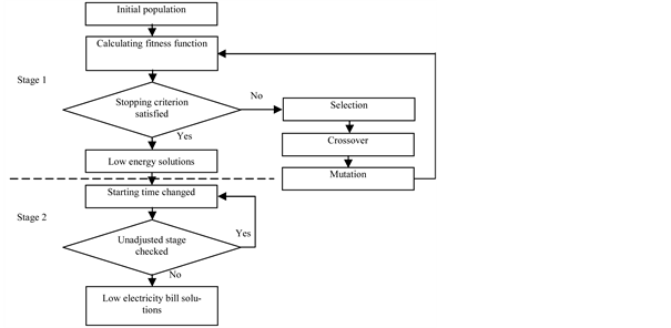
Figure 2. Flow chart of solving procedure of ESGA.
3.1. The First Stage of ESGA
This study utilized two genetic algorithms for solving problems: the CGA for minimizing the makespan and calculating the electricity cost and EGA for determining low energy consumption scheduling and calculating the electricity cost concurrently [6] . The procedures of the proposed method are demonstrated as follows:
3.1.1. Encoding
According to Dai et al. [6] , a job set, stage set, and machine set ( ) are present at each stage. This study formulated FFS scheduling as a genetic matrix in which the columns are jobs and stages are rows.
(12)
The is a real number in the interval (1, ). indicates which machine processes job j, and the decimal indicates the processing sequence; the lower the decimal is, the earlier the job is processed. A coding matrix represents a chromosome in which genes are present.
(13)
For example, in FFS scheduling, the coding matrix consists of three stages, in which there are two machines and eight jobs to be processed.
(14)
Row 1 represents processing conditions of the first stage. The means processed in machine 1, means processed in machine 2, and means processed in machine 1. The decimal of is 0.301smaller than 0.415 of , which represents is processed earlier than .
(15)
3.1.2. Initial Population
The initial solution is the first population of a genetic algorithm. Generally, two methods can generate initial solutions: one is randomly generated and other requires research. The scale of the initial population affects the efficiency and quality of solutions. A random initial solution was used in this study.
3.1.3. The Fitness Function
The fitness function can identify the quality of chromosomes, enabling inferior solutions to be screened out. The fitness function of the CGA is as follows:
(16)
The fitness function of EGA is as below:
(17)
3.1.4. Selection
The algorithm selects a favorable parent from chromosomes and proceeds with crossover and mutation. Each chromosome has a fitness value, which determines the possibility for crossover and mutation. This study adopted roulette wheel selection.
3.1.5. Crossover
The proposed algorithm partially exchanges two chromosomes. In this study, the exchange rate was set as, which is a rounded-up approximation of the quantity of exchanged chromosome multiplied by the exchange rate. If the quantity of exchanged chromosome is odd, then one chromosome is added to the total chromosomes and the quantity becomes even. The exchange rate was set at 0.9, and this study adopted a two-point crossover method to solve the considered problem.
3.1.6. Crossover
Mutation can generate multiple and various children. A mutation rate of was set in this study. The proposed method arbitrarily generates a probability value. If the value is below the mutation rate, mutation occurs. The mutation rate was set at 0.1. The mutation rate is uniformly distributed from 0 to 1. If the rate becomes 1, the proposed algorithm regenerates an interval of real numbers (1, Ms + 1).
3.2. The Second Stage of ESGA
Although the genetic algorithm generates scheduling with lower electricity costs, some jobs still generate high electricity costs. The solutions generated from the GCA and EGA in the first stage were adjusted using the ACGA, and problems in the second stage were solved using the AEGA to avoid high-energy price periods.
The adjustment rule begins from the final stage and proceeds in descending order. The proposed approach organizes the operations into the final order. The method gradually schedules operations in the off-peak period and moves the sequence of operation away from the on-peak period until all jobs are scheduled. Figure 3 illustrates the flow chart.
3.3. A Brief Example
In a job scheduling scheme consisting of three stages, two machines at each stage, and eight jobs to be processed, the total working time is 16 hours and the factory working period is from 6 a.m. to 10 p.m. on each day. Table 1 shows the operation time:
Table 2 shows the consumed energy of machines. The starting time of the machines is assumed to be short with sudden turn-on energy consumption.
Table 3 shows the electricity costs of every time period. The parameters of the proposed method are as follows: initial population, 30; exchange rate, 0.9; mutation rate, 0.1; and stopping criterion, 300 iterations.
3.3.1. The First Stage of ESGA
Figure 4 shows the computational result using CGA, and the electricity bill is NT$ 3277.8.

Figure 3. Flow chart of solving procedure of ESGA.

Table 1. The operation working time.
Table 2. The operation working time.
Remarks: This study assumes the starting time of machine is short with a sudden turn-on energy consumption.
Figure 5 shows the computational result using EGA, and the electricity bill is NT$ 2900.6.
3.3.2. The Second Stage of ESGA
The adjustment rule begins from the final stage and proceeds in descending order. The proposed approach organizes operations into the final order. The method gradually schedules operations in the off-peak period and moves the sequence of operation away from the on-peak period until all jobs are scheduled. Figure 6 shows the computational result obtained using the ACGA and the electricity cost is NT$ 2929.7.
Figure 7 the computational result using AEGA, and the electricity bill is NT$ 2807.4.
Table 4 lists four computational results obtained using the CGA as the
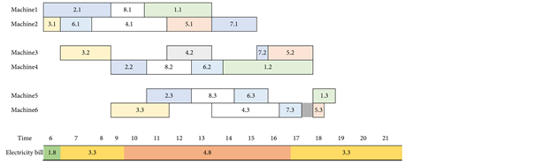
Figure 4. The Gantt chart of computational result using CGA.

Figure 5. The Gantt chart of computational result using EGA.
Table 3. The electricity bill of time periods.
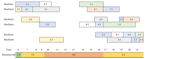
Figure 6. The Gantt chart of computational result using ACGA.
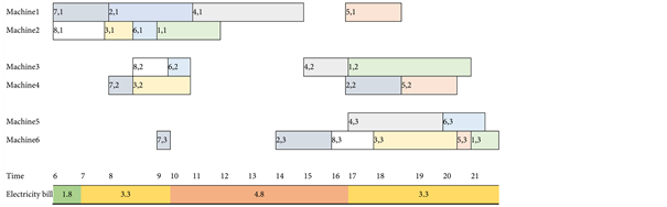
Figure 7. The Gantt chart of computational result using AEGA.
Table 4. Comparison of electricity bills.
benchmark for comparison. According to Table 4, applying the CGA generates the highest electricity cost, because it neglects the costs of standby, shutdown, and different time periods. Furthermore, the EGA considers different conditions of machines and can lower the electricity cost; however, jobs are processed in the on-peak period. The proposed method using ESGA can efficiently avoid processing jobs in the on-peak period. Moreover, ESGA can lower the electricity cost by up to 11% and 14%, respectively, compared with the CGA. The results demonstrate higher energy saving with the AEGA than with the CGA, EGA, and ACGA.
4. Computational Experiments
All tests were conducted on a PC with an Intel® Core™ i5-4300U 1.9-GHz CPU with 8 GB of RAM. The operation system used was Windows® 8.1. The FFS scheduling problem is . The parameters of the proposed method are the number of jobs, type of stage, number of machines, energy consumption of machines, processing time of jobs, and due dates. For the considered problems, the number of jobs was 30, 60, or 90; the type of stage was 3 or 5; and the number of machines in the two stages = 6, 9. Table 2 and Table 5 show the energy consumption of machines. Moreover, the processing time of jobs was limited within U [2] [9] ; the unit time was 30 minutes; the factory working period was from 6 a.m. to 10 p.m. on each day; and the electricity costs of various time periods are shown in Table 3. The formula of the due date , among which the represents the average processing time of machines, and TF is the tardy factor; Type I was 0.3 and Type II was 0.5. The working duration per day was assumed to be 16 hours. Therefore, when the formula of the due date provided a duration of 20 hours, the due date was estimated to be 2 days. Finally, the parameters of the genetic algorithms were set on the basis of a pretest to improve the results; specifically, the initial population was 30; the exchange rate was 0.9; the mutation rate was 0.1; and the stopping criterion was 500 iterations.
4.1. Analysis of Effectiveness
To assess the effectiveness of the proposed algorithm in solving the considered problems, 12 conditions were applied to randomly test 30 generated problem sets; specifically, the number of jobs was 30, 60, or 90; the type of stage was 3 or 5; and the number of machines in the two stages was 6 or 9. Table 6 provided a comparison of the average solutions and average solving times of the CGA, EGA, ACGA, and AEGA for efficacy analysis under Type I of slacker due dates.
Table 7 provided a comparison of the average solutions and average solving times of the CGA, EGA, ACGA, and AEGA for efficacy analysis under Type II of non-slacker due dates.
Table 6 and Table 7 illustrate that for different due dates, the cost of energy consumption is lower for the ACGA and AEGA than for the CGA. Type I has slacker due dates than those of Type II, indicating that the EGA and AEGA provide superior solutions. A data set of 30/6/5 has the same due date as that of Type I and Type II; therefore, the improvement is not remarkable. The CGA calculates the electricity cost for the minimal makespan; therefore, the CGA and ACGA might not provide superior solutions in the Type I condition. Table 8 show comparison cost ratios for electricity costs obtained using all methods under Type I of slacker due dates.
Table 8 and Table 9 show comparison cost ratios for electricity costs obtained using all methods under Type I of non-slacker due dates.
Table 5. The energy consumption during three time periods of 5-stage machines.
Table 6. The effectiveness of time window Type I.
Remarks: The unit cost is NT$.
Table 7. The effectiveness of time window Type II.
Remarks: The unit cost is NT$.
Table 8 and Table 9 illustrate that the EGA, ACGA, and AEGA yielded lower electricity costs than did the CGA. Moreover, the AEGA provided solutions superior to those of the ACGA method in terms of effectiveness.
4.2. Analysis of Robustness
To assess the robustness of the proposed algorithms in solving the considered problems, 12 conditions were applied to test the same solution 30 times;
Table 8. The comparison costs ratio of electricity bills of time window Type I.
Table 9. The comparison costs ratio of electricity bills of time window Type II.
specifically, the number of jobs was 30, 60, or 90; the type of stage = 3, 5; and the number of machines in the two stages = 6, 9. Table 10 and Table 11 provide a comparison of the average solutions, optimal solutions, and poorest solutions calculated using the CGA, EGA, ACGA, and AEGA in the analysis of robustness.
The test results in Table 10 and Table 11 for robustness show that the ACGA and AEGA are affected by original solutions during adjustment procedures,
Table 10. The robustness of time window Type I.
Remarks: The unit cost is NT$.
causing the electricity cost to decrease partially. Thus, the robustness of the proposed method was fairly identified.
5. Computational Experiments
This study investigated the use of limited resources of parallel machines to promote practical production and environmental protection. Ideal practical production for better energy using effective scheduling prevents processes from excessive energy consumption and energy price fluctuations. Recent studies on sustainable manufacturing focused on energy saving to reduce the unit production cost and environmental impacts.
Most importantly, the application of the optimization of the scheduling can be respected for costs down and energy-saving simultaneously. Under an operational environment in which electricity costs differ depending on the time period, manufacturing activities in machine shops increase electricity consumption costs. In particular, machine conditions and job processing time periods are crucial factors in making energy-saving decisions during the manufacturing process.
Table 11. The robustness of time window Type II.
Remarks: The unit cost is NT$.
According to the analysis, the CGA, EGA, ACGA, and AEGA can efficiently solve problems. The electricity cost ratio for the CGA, EGA, ACGA, and AEGA is 1:0.78:0.95:0.74, demonstrating that the AEGA can efficiently solve the problem. The robustness test results show that the ACGA and AEGA of ESGA are affected by original solutions during adjustment procedures and partially reduce electricity costs. Thus, the robustness of the proposed method was appropriately identified. As a whole, the proposed method can lower electricity bills to fit green energy nowadays.
Finally, enterprises can adopt the proposed method for enhancing practical production in the flexible job shop scheduling environment and generate profits by fully exploiting the advantages of the method in the future. In addition, the proposed method can mitigate the environmental impact of manufacturing processes and protect environment at the same time.
Cite this paper
Huang, R.-H., Yu, S.-C. and Chen, P.-H. (2017) Energy-Saving Scheduling in a Flexible Flow Shop Using a Hybrid Genetic Algorithm. Journal of Environmental Protection, 8, 1037-1056. https://doi.org/10.4236/jep.2017.810066
References
- 1. Goldratt, E.M. and Cox, J. (1984) The Goal: Excellence in Manufacturing. North River Press, Great Barrington, MA.
- 2. Tongur, V. and ülker, E. (2014) Migrating Birds Optimization for Flow Shop Sequencing Problem. Journal of Computer and Communications, 2, 142-147. https://doi.org/10.4236/jcc.2014.24019
- 3. Zabihzadeh, S.S. and Rezaeian, J. (2016) Two Meta-Heuristic Algorithms for Flexible Flow Shop Scheduling Problem with Robotic Transportation and Release Time. Applied Soft Computing, 40, 319-330. https://doi.org/10.1016/j.asoc.2015.11.008
- 4. Linn, R. and Zhang, W. (1999) Hybrid Flow Shop Scheduling: A Survey. Computers and Industrial Engineering, 37, 57-61. https://doi.org/10.1016/S0360-8352(99)00023-6
- 5. Ribas, I., Leisten, R. and Framiñan, J.M. (2010) Review and Classification of Hybrid Flow Shop Scheduling Problems from a Production System and a Solutions Procedure Perspective. Computers & Operations Research, 37, 1439-1454. https://doi.org/10.1016/j.cor.2009.11.001
- 6. Dai, M., Tang, D., Giret, A., Salido, M.A. and Li, W.D. (2013) Energy-Efficient Scheduling for a Flexible Flow Shop Using an Improved Genetic-Simulated Annealing Algorithm. Robotics and Computer-Integrated Manufacturing, 29, 418-429. https://doi.org/10.1016/j.rcim.2013.04.001
- 7. Huang, R.H., Yu, S.C. and Kuo, C.W. (2014) Reentrant Two-Stage Multiprocessor Flow Shop Scheduling with Due Windows. The International Journal of Advanced Manufacturing Technology, 71, 1263-1276. https://doi.org/10.1007/s00170-013-5534-4
- 8. Mukund Nilakantan, J., Huang, G.Q. and Ponnambalam, S.G. (2015) An Investigation on Minimizing Cycle Time and Total Energy Consumption in Robotic Assembly Line Systems. Journal of Cleaner Production, 90, 311-325. https://doi.org/10.1016/j.jclepro.2014.11.041
- 9. Zhang, H., Zhao, F., Fang, K. and Sutherland, J.W. (2014) Energy-Conscious Flow Shop Scheduling under Time-of-Use Electricity Tariffs. CIRP Annals-Manufacturing Technology, 63, 37-40. https://doi.org/10.1016/j.cirp.2014.03.011
- 10. Setlhaolo, D., Xia, X. and Zhang, J. (2014) Optimal Scheduling of Household Appliances for Demand Response. Electric Power Systems Research, 116, 24-28. https://doi.org/10.1016/j.epsr.2014.04.012
- 11. Jin, W., Hu, Z. and Chan, C. (2017) An Innovative Genetic Algorithms-Based Inexact Non-Linear Programming Problem Solving Method. Journal of Environmental Protection, 8, 231-249. https://doi.org/10.4236/jep.2017.83018
- 12. Mouzon, G., Yildirim, M.B. and Twomey, J. (2007) Operational Methods for Minimization of Energy Consumption of Manufacturing Equipment. International Journal of Production Research, 45, 4247-4271. https://doi.org/10.1080/00207540701450013
- 13. Fang, K., Uhan, N., Zhao, F. and Sutherland, J.W. (2011) A New Approach to Scheduling in Manufacturing for Power Consumption and Carbon Footprint Reduction. Journal of Manufacturing Systems, 30, 234-240. https://doi.org/10.1016/j.jmsy.2011.08.004
- 14. Tibi, N.A. and Arman, H. (2007) A Linear Programming Model to Optimize the Decision-Making to Managing Cogeneration System. Clean Technologies and Environmental Policy, 9, 235-240. https://doi.org/10.1007/s10098-006-0075-2
- 15. He, Y., Li, Y.F., Wu, T. and Sutherland, J.W. (2015) An Energy-Responsive Optimization Method for Machine Tool Selection and Operation Sequence in Flexible Machining Job Shops. Journal of Cleaner Production, 87, 245-254. https://doi.org/10.1016/j.jclepro.2014.10.006
- 16. Bruzzone, A.A.G., Anghinolfi, D., Paolucci, M. and Tonelli, F. (2012) Energy-Aware Scheduling for Improving Manufacturing Process Sustainability: A Mathematical Model for Flexible Flow Shops. CIRP Annals-Manufacturing Technology, 61, 459-462. https://doi.org/10.1016/j.cirp.2012.03.084
- 17. Shao, W., Pi, D. and Shao, Z. (2017) Memetic Algorithm with Node and Edge Histogram for No-Idle Flow Shop Scheduling Problem to Minimize the Makespan Criterion. Applied Soft Computing, 54, 164-182. https://doi.org/10.1016/j.asoc.2017.01.017
- 18. Lian, Z.G. (2010) A Local and Global Search Combine Particle Swarm Optimization Algorithm for Job-Shop Scheduling to Minimize Makespan. Discrete Dynamics in Nature and Society, 2010, Article ID 838596, 11 p.
- 19. Zhang, C.S., Ning, J. and Ouyang, D. (2010) A Hybrid Alternate Two Phases Particle Swarm Optimization Algorithm for Flow Shop Scheduling Problem. Computers and Industrial Engineering, 58, 1-11. https://doi.org/10.1016/j.cie.2009.01.016
- 20. Liu, H.C., Gao, L. and Pan, Q. (2011) A Hybrid Particle Swarm Optimization with Estimation of Distribution Algorithm for Solving Permutation Flowshop Scheduling Problem. Expert Systems with Applications, 38, 4348-4360. https://doi.org/10.1016/j.eswa.2010.09.104
- 21. Zhao, F., Tang, J., Wang, J. and Jonrinaldi, J. (2014) An Improved Particle Swarm Optimisation with a Linearly Decreasing Disturbance Term for Flow Shop Scheduling with Limited Buffers. International Journal of Computer Integrated Manufacturing, 27, 488-499. https://doi.org/10.1080/0951192X.2013.814165
- 22. Li, T., Castro, P.M. and Lv, Z. (2017) Life Cycle Assessment and Optimization of an Iron Making System with a Combined Cycle Power Plant: A Case Study from China. Clean Technologies and Environmental Policy, 19, 1133-1145. https://doi.org/10.1007/s10098-016-1306-9
- 23. Ma, B. and Yu, Y. (2017) Industrial Structure, Energy-Saving Regulations and Energy Intensity: Evidence from Chinese Cities. Journal of Cleaner Production, 141, 1539-1547. https://doi.org/10.1016/j.jclepro.2016.09.221
- 24. Peyramalea, V. and Wetzelb, C. (2017) Analyzing the Energy-Saving Potential of Buildings for Sustainable Refurbishment. Procedia Environmental Sciences, 38, 162-168. https://doi.org/10.1016/j.proenv.2017.03.098
- 25. Moon, J.Y., Shin, K. and Park, J. (2013) Optimization of Production Scheduling with Time-Dependent and Machine-Dependent Electricity Cost for Industrial Energy Efficiency. The International Journal of Advanced Manufacturing Technology, 68, 523-535. https://doi.org/10.1007/s00170-013-4749-8
- 26. Shrouf, F., Ordieres-Mere, J., Garcia-Sanchez, A. and Ortega-Mier, M. (2014) Optimizing the Production Scheduling of a Single Machine to Minimize Total Energy Consumption Costs. Journal of Cleaner Production, 67, 197-207. https://doi.org/10.1016/j.jclepro.2013.12.024
- 27. Pinedo, M.L. (2008) Scheduling: Theory, Algorithm and Systems. 3rd Edition, Springer-Verlag, New York.