Journal of Environmental Protection
Vol. 3 No. 8A (2012) , Article ID: 21780 , 11 pages DOI:10.4236/jep.2012.328094
Coliform Bacteria: The Effect of Sediments on Decay Rates and on Required Detention Times in Stormwater BMPs
![]()
1Department of Civil Engineering, Environmental Engineering Program, The University of Mississippi, Oxford, USA; 2Department of Civil Engineering, The University of Mississippi, Oxford, USA.
Email: *csurbeck@olemiss.edu
Received June 2nd, 2012; revised July 4th, 2012; accepted August 5th, 2012
Keywords: fecal indicator bacteria; decay rate; sediment; nutrients; organic carbon; best management practices (BMPs)
ABSTRACT
Fecal indicator bacteria, such as total coliforms and E. coli, are a challenge to control in urban and rural stormwater runoff. To assess the challenges of improving bacterial water quality standards in surface waters, microcosm experiments were conducted to assess how decay rates of total coliforms and E. coli are affected by sediments and associated organic matter. Samples were collected at a lake embayment to create laboratory microcosms consisting of different combinations of unsterilized and sterilized water and sediment. Calculated first-order decay rate constants ranged from 0.021 to 0.047 h−1 for total coliforms and 0.017 and 0.037 h−1 for E. coli, depending on how each microcosm was prepared. It is evident that sediment in contact with the water column decreases bacteria decay rate, showing that care should be taken when designing stormwater treatment measures. In addition, high organic carbon content in the sediment temporarily increased bacteria concentrations in the water column. The results demonstrate that stormwater treatment measures, such as extended detention basins and constructed wetlands, must hold water for several days to allow for reduction of bacterial concentrations to acceptable levels. In addition, to troubleshoot detention basins and constructed wetlands for causes of high effluent bacterial concentrations, analyses of sediment, organic carbon, and water column depth should be conducted.
1. Introduction
The presence of fecal indicator bacteria (FIB) in surface waters can have detrimental consequences to human and economic health. For example, exceedingly high occurrences of these bacteria in recreational beaches can put bathers at risk of contracting illnesses. As a prevention to illnesses, beaches are closed, resulting in economic losses in municipalities that depend on tourism [1,2]. To protect recreation and ecosystems in water bodies, the United States’ Clean Water Act 303(d) impaired waters list includes thousands of creeks, rivers, and coastal zones classified as impaired for pathogens [3]. The denotation of “pathogens” includes known pathogenic organisms but, more commonly, FIB, such as total coliforms, fecal coliforms, Escherichia coli (E. coli), and enterococci bacteria. A large contributor to FIB in surface waters is stormwater runoff [4,5]. Solutions to controlling pollution to surface waters from stormwater runoff are called Best Management Practices (BMPs), also known as Stormwater Control Measures (SCMs), and include a range of strategies from educating the public to cleaning animal feces from paved surfaces to constructing stormwater treatment detention basins and wetlands. However, current efforts to reduce concentrations of FIB using stormwater BMPs have yielded inconsistent results. Monitoring efforts of BMP inlet and outlet points during storms generally report minor decreases or even increases of FIB at the outlets [6]. Some monitoring efforts of the same type of BMP but in different locations yield opposite results [7], and some BMPs perform well in all seasons except summer [8].
Reasons for inconsistent results in treating FIB with BMPs are the complexities associated with this type of pollutant. The experiments reported in this paper give insight on what may be necessary for structural BMPs, such as extended detention basins and constructed wetlands, to effectively reduce FIB. An extended detention basin is a constructed pond used to detain excess stormwater runoff as well as promote settling of various pollutants found in runoff. As the stormwater runoff is detained in the basin, sedimentation promotes the reduction of total suspended solids (TSS) and other pollutants attached to suspended solids. A constructed wetland is used in a similar manner to the extended detention basin, but it uses plants to aid in the reduction of TSS, FIB, organic materials, and nutrients in the water.
Bed sediments have the potential to increase FIB concentrations in the water column by furnishing nutrients and additional FIB but may decrease water column FIB by providing a source of predator organisms. In this study we examined how FIB concentrations behave in the water column when bed sediments are present. We hypothesized that the decay rate of FIB in the water column, and therefore in structural BMPs, decreases with the presence of bottom sediments. We used microcosm studies to experimentally determine FIB decay rates for five treatments that provided input into reasons for FIB decay in the water column and the effect of sediments. Further, we estimated the hydraulic residence time necessary in an extended detention basin and constructed wetland to reduce total coliform concentrations to an acceptable level, based on the decay rates from the experiments.
This research builds on literature that considers the impact of sediments and associated organic matter and nutrients on water quality. Organic matter and nutrients in the water column can impact the occurrence of FIB, whether the nutrients come from sediment or another source. For example, Smith and Prairie [9](Smith and Prairie 2004) studied the effect of dissolved organic carbon (DOC) and nutrients on the behavior of bacteria in different types of lakes. They found that bacteria growth rates were positively correlated with total phosphorus concentrations and that DOC usage by lake bacteria depends strongly on the availability of phosphorus; the combination of carbon and phosphorus produced significantly greater bacteria concentrations than phosphorus alone. Similar results were found by Surbeck et al. [10], but the bacteria were FIB in a concrete-lined urban river where the source of phosphorus and organic carbon was not sediment, but the discharge from a wastewater treatment plant. Additionally, Jeng et al. [11] found that indicator organisms entered an estuary through stormwater runoff and settled to the bottom sediments, experiencing prolonged survival. Bolster et al. [12] were able to increase concentrations of E. coli in laboratory experiments of estuarine waters with high nutrient content.
Microcosm studies on FIB have been used by Craig et al. [13] and consisted of intact sediment cores taken from coastal areas with distinct sediment characteristics to determine the decay rates of E. coli in water and sediment. It was found that E. coli persisted in sediment, compared with overlying water. Small particle size and high organic carbon content were found to enhance survival; that is, sediments containing high proportions of clay and nutrients are more conducive to survival than sandy sediments.
2. Materials and Methods
2.1. Sample Collection
Water and sediment samples were collected during four events from an embayment (the flooded mouth of a tributary stream) contiguous with a manmade lake in northern Mississippi, USA. Water and sediment were collected from this water body and used in laboratory microcosms to simulate performance of BMPs with high FIB loadings.
The water and sediment samples were collected in Nalgene bottles (Nalgene Company, Rochester, NY) previously autoclaved at 121˚C in an EZ 9 autoclave (2340EA, Tuttnauer, Hauppauge, NY). Sediment samples were collected with 2-inch by 4-inch aluminum sediment core sleeves previously autoclaved at 134˚C. The sleeve was filled approximately halfway so that the sediment would represent the top 5 cm, which contains the most recent nutrient influx [14]. A sediment particle size analysis [15] was performed on the sediment and yielded size fractions of 71% sand and 29% silt.
Water samples were collected from the embayment surface, and sediment samples were collected from a submerged portion of the bank on four dates following precipitation events (Table 1). All samples were transported on ice, and microcosm set-up began once the samples were brought to the laboratory at the University of Mississippi.
2.2. Pre-Microcosm Preparation and Microbiological Analyses
The sediment was mixed to make a homogeneous soil matrix in order to provide each microcosm with similar sediment characteristics. This was accomplished by putting the sediment from the Nalgene bottles in an aluminum pan and manually mixing. Afterwards, sediment for two of the microcosms was sterilized by autoclaving at 121˚C.
Next, bacteria were extracted from the unsterilized sediment within three hours of collection. This was done following a procedure adapted from Craig et al. [16] and Jeong et al. [17]. Once the supernatant of the extraction procedure was retrieved, it was processed for analysis of total coliform and E. coli, in duplicate, using the defined-substrate method Colilert (IDEXX Laboratories, Inc., Westbrook, ME), in units of most probable number (MPN) per kg, and recorded. FIB analysis was performed on water samples using the Colilert method, but with concentration results in units of MPN per 100 ml (or 1
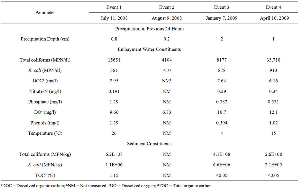
Table 1. Summary of initial concentrations of constituents in embayment water and sediment used for microcosm studies.
deciliter, dl). Colilert is known as Standard Method 9223 [18].
2.3. Microcosm Preparation
Following the sediment preparation and FIB quantification described above, seven microcosms were set up in 500-ml glass Erlenmeyer flasks. When necessary, water was filter-sterilized with a 0.22-micron filter (Model number 8532, Corning, Corning, NY). Sediments were sterilized by autoclaving. The microcosms were incubated in a shaker incubator (Classic C24, New Brunswick Scientific, Edison, NJ) rotating at 60 rpm to prevent settling of FIB, while mimicking the slow movement of water in a detention basin or constructed wetland. The shaker incubator was stopped for sample collection, but bacterial settling would not have occurred in the few minutes in which the shaker was stopped. An incubation temperature of 30˚C was used for all experiments as a representation of a summertime (i.e., recreation) water temperature. The incubator had a glass cover and was located near a window, exposing the microcosms to sunlight during the daytime.
Figure 1 is an illustration of Microcosms 1 through 5, which are described next. Microcosm 1 was composed of embayment water alone and was used to monitor FIB die-off free from the influence of bed sediment. Microcosm 2 was composed of embayment water and bottom sediment. This combination simulated natural conditions and was used to monitor FIB in the water as affected by nutrients associated with the water and nutrients and FIB
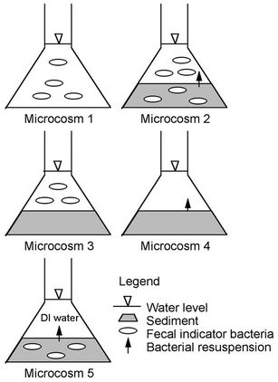
Figure 1. Schematics demonstrating initial location of FIB in microcosms. Two control microcosms are excluded from the figure.
associated with the sediment. Microcosm 3 was composed of embayment water and autoclaved sediment and was used to monitor FIB in water under the effect of nutrients in the water and the sediment, but not FIB from the sediment. Microcosm 4 was composed of sediment and filter-sterilized embayment water. It was used to monitor FIB in water that resuspended from sediments and that was affected by nutrients in water and sediment. Microcosm 5 was composed of sediment and sterilized deionized (DI) water and was used to monitor FIB in water associated with FIB resuspension from sediment without the effect of FIB and nutrients from the water. Microcosm 6 was composed of sterilized embayment water and was used as a control to monitor whether filter-sterilizing the water was successful in removing FIB. Microcosm 7 was composed of sterilized DI water and sterilized sediment and was used as a control to monitor whether autoclaving the sediment and filter sterilizing the DI water were successful in removing FIB.
Each sediment-water microcosm consisted of approximately 200 g of sediment and 300 to 500 ml of water. The volumes of microcosms of water alone were between 230 to 500 ml.
2.4. Microcosm Monitoring
Data were collected for four events, each consisting of seven unique microcosms. During the microcosm study events, aliquots of 1 mL of water in the microcosms were collected at twelve-hour intervals in the first two days, and aliquots of 10 mL of water were collected at 24-hour intervals in the subsequent five days. Each aliquot of water was analyzed for FIB following the procedures described previously.
2.5. Chemical Analyses
Water samples, sediment samples, and microcosm samples were also analyzed for chemical water quality parameters. Those analyses and the times during which they were conducted are described below.
Organic Carbon. At the beginning of each study, a grab sample of water and soil were collected and kept refrigerated until the study was completed. At the time of collection, water samples were filtered through a 0.45-micron filter (Millipore, Billerica, MA) in a 500-ml capacity filtration kit (Nalgene Company, Rochester, NY). Samples of water and sediment taken from the end of the microcosm studies were shipped on ice overnight to Environmental Testing and Consulting, Inc. (ETC) in Memphis, TN, who analyzed water samples for total organic carbon (TOC) using Standard Method SM-5310B [18]. Sediment samples were analyzed for organic carbon using the Walkley-Black method [19]. Because the water samples were filtered prior to the laboratory analysis, the results are reported as DOC.
Dissolved Oxygen, Phenols, Nitrate, and Phosphate. The water samples were tested before and after the microcosm studies for dissolved oxygen, phenols, nitrate, and phosphate using a V-2000 Multi-Analyte Photometer and vacu-vial kits (CHEMetrics, Calverton, VA).
2.6. Data Analysis
Monitoring of the seven microcosms over four events yielded concentrations of total coliform and E. coli in the water column over 7 days. For Microcosms 2, 3, 4, and 5, FIB concentrations were adjusted to compensate for the changing ratio of sediment to water. That is, during the monitoring of microcosms, as aliquots of water were removed for analysis of FIB, the volume of water inside the microcosms decreased, increasing the sediment-towater volume and mass ratios. Because this study was driven by the hypothesis that sediment influenced the concentrations of FIB in water, and because experimentally the sediment became more influential due to the decreasing volume of water as aliquots were removed during the seven days, it was necessary to perform an adjustment calculation for the concentration of FIB in the water column (Ct). The following assumptions were used to determine the adjustment calculations for the changing sediment-to-water ratio: 1) the FIB concentrations in the water column are affected in direct proportion to the sediment; 2) the partitioning properties were not affected with the changing ratios; 3) FIB in the water did not settle into the sediment because of the turbulence in the water due to the mechanical shaking; and 4) FIB and/or nutrients could resuspend from the sediment into the water column. To conduct the adjustment, the concentration of FIB measured in each aliquot at time t (Caliquot,t) was multiplied by the volume of water existing at the time of the aliquot collection (Vt) and then divided by the initial volume of water in the microcosm (Vo), as shown in Equation (1).
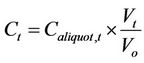 (1)
(1)
Vt/Vo ranged from 1.0 at t = 0 to 0.72 at t = 7 days. Following this adjustment calculation for the microcosms containing sediment and water, the concentrations were normalized for Microcosms 1 through 5 by dividing each Ct by the initial concentration, Co, as per Equation (2).
 (2)
(2)
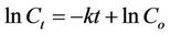
This normalization allowed all of the initial concentrations to be equal to 100 and allowed all four events to be analyzed together. Further, the natural logarithms of the normalized concentrations were plotted against time to establish first-order decay rate constants in base e using the slope value of a best-fit line. This is described by Equation (3),
 (3)
(3)
where C is concentration, t is time, and k is the first-order decay rate constant. If C = Co at t = 0, then this equation can be integrated by separation of variables to yield the linear equation
 (4)
(4)
where lnCt is the dependent variable, t is the independent variable, k is the slope of the line, and lnCo is the y-intercept. Best-fit line calculations with slope, y-intercept, standard deviations, and the Pearson correlation coefficient were calculated using the software Igor Pro 5.01 (WaveMetrics, Inc., Lake Oswego, OR). The significance of the correlations was calculated using the SPSS Statistics 15 (SPSS, Inc., Chicago, IL). For this analysis, where FIB concentrations were lower than the detection limit, the value of half of the detection limit was used. FIB concentrations above quantification limits occurred only in Microcosm 3, and this microcosm was excluded from this analysis.
2.7. Applications to Stormwater Best Management Practices
The calculated total coliform decay rates for the different microcosms were used to evaluate the time and the surface area necessary for stormwater BMPs, such as extended detention ponds and constructed wetlands, to detain stormwater until coliform concentrations decreased to an acceptable level.
In order to calculate the detention times necessary for a BMP to reduce concentrations of total coliforms, the decay rate constant calculated for Microcosms 1 and 2 were used based on certain assumptions. For the extended detention pond, the total coliform decay rate for Microcosm 1 was used because the depth of a detention pond would be large enough that the bottom sediments have little effect on the decay rates of total coliform in the water detained. To calculate the detention times for a constructed wetland to decrease FIB concentrations, the total coliform decay rate constant for Microcosm 2 was utilized because this microcosm set up was similar to a wetlands BMP in that the water levels in wetlands are shallow. Then it can be assumed that sediment will have an effect on the water by becoming a source of resuspended coliforms and/or nutrients, providing a decreased decay rate of coliforms. By varying the initial concentration of FIB from 10,000 MPN/dl to 1000 MPN/dl, Equation 4 was rearranged to calculate the time, t, needed to reach a final FIB concentration of 330 MPN/dl. While there is no ambient water quality criteria for total coliforms, this concentration was used as an example standard from a total maximum daily load (TMDL) calculation from New York State [H20H].
Following the calculation of the detention times, the necessary area to be occupied by an extended detention pond and constructed wetland was calculated with the assumption of a known BMP depth of 3 m for a detention pond and 0.20 m for a constructed wetland and a first flush depth of 1 inch (2.54 cm) of runoff from the drainage area. A first flush volume was then calculated, equal to 2.54 cm multiplied by drainage areas ranging from 16,200 to 80,900 m2. The drainage areas were varied in order to visualize the consequent first flush volumes and the necessary required area of the detention pond. The surface area occupied by the BMP then was the first flush volume divided by the assumed water depth of the BMP. Note that this is not a design procedure for detention ponds and constructed wetlands, but rather a simple calculation to estimate dimensions, especially when the first flush occurs in a small interval of time, say, 1 hour.
3. Results
As a recreational water body, the sampling station does not meet standards for E. coli, exceeding the limit of 126 MPN/dl [H21H] in three events, of which two are during swimming months. The concentrations of the water quality parameters collected are shown in Table 1. This table also shows that some precipitation occurred within 24 hours prior to each sampling event, but water quality parameters were not correlated with antecedent precipitation depth. Concentrations of FIB and TOC in sediment samples varied among events and are further discussed below.
3.1. Evaluation of Fecal Indicator Bacteria Decay Rates in the Microcosms
Results of the first-order decay best-fit lines combining all four events for Microcosms 1, 2, 4, and 5 are shown in Figure 2. The axis range for each plot is the same, so the best-fit lines (solid for total coliform and dashed for E. coli) can be compared for steepness. The best-fit line for Microcosm 1, composed of embayment water alone, had the steepest slope k, showing that FIB decay is faster when sediment is not present. A comparison of the decay constants of these four microcosms, combining all four events, is shown in Table 2. It is evident that FIB decay was faster in Microcosms 1 (embayment water alone) and 2 (embayment water and sediment) than in 4 (sediment and sterilized embayment water) and 5 (sediment and sterilized DI water). Calculated standard deviations for k varied from 1 to 48 percent of the calculated k. The Pearson correlation coefficients R ranged from −0.41 to
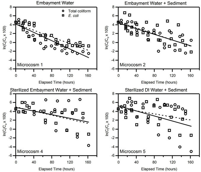
Figure 2. Plots of normalized FIB concentrations versus time for Microcosms 1, 2, 4, and 5, with data from all four microcosm sampling events. The solid line is the best-fit line for total coliforms; the dashed line is the best-fit line for E. coli.
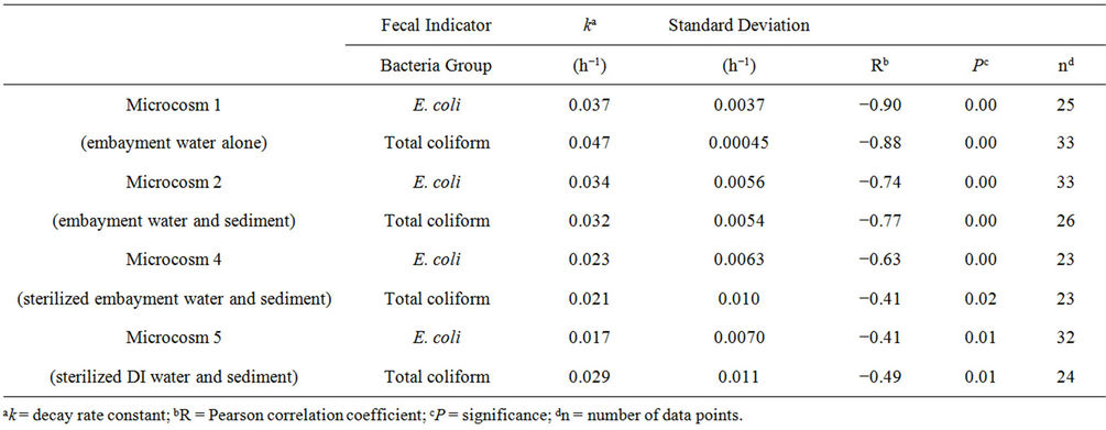
Table 2. Decay rate constants and statistics for Microcosms 1, 2, 4, and 5, calculated from the four microcosm events combined.
−0.88 and were highest for Microcosms 1 and 2. All correlations were significant at . Microcosms 6 and 7 were negative control microcosms, and all FIB concentrations were below detection limits, demonstrating that the sterilization methods were effective.
Microcosm 3, composed of embayment water and sterilized sediment, was to be evaluated in the same manner as Microcosms 1, 2, 4, and 5. However, data from this microcosm were excluded from the evaluation because FIB concentrations increased rather than decayed (Table 3). Plots are not shown for this microcosm because several concentrations were above upper quantification limits. Microcosm 3 was created to demonstrate how FIB would behave in water affected by nutrients suspending from the sediment when FIB were not present in sediment. To set up Microcosm 3, the sediment was autoclaved at 121˚C for 1 hour and then added to the flask, followed by the addition of water. This microcosm
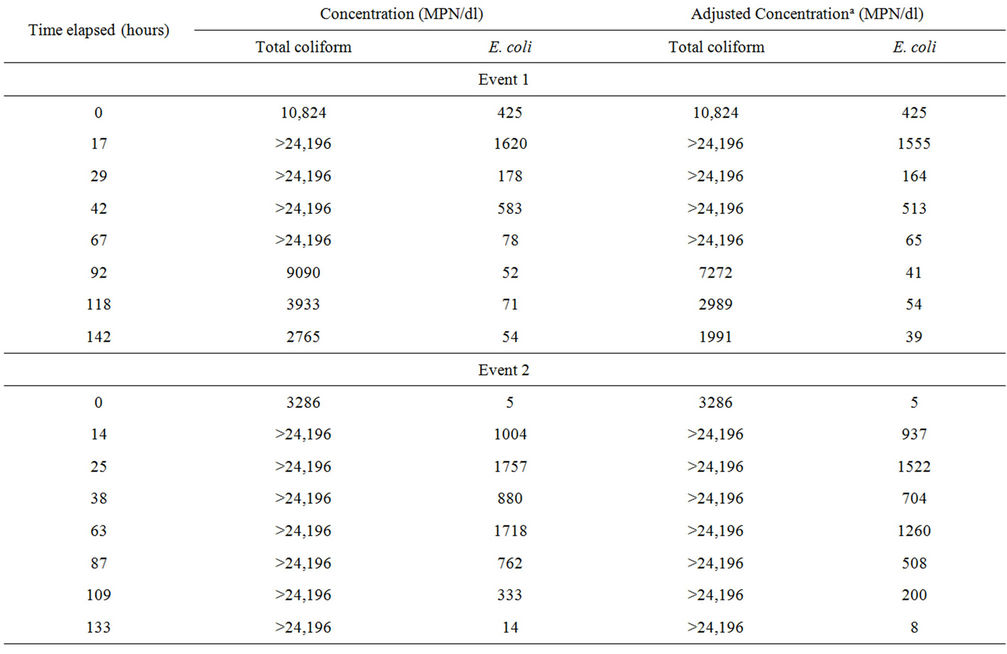
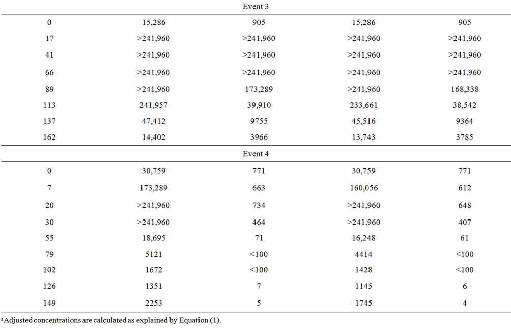
Table 3. Fecal indicator bacteria concentrations in Microcosm 3 during the four events.
was then monitored with the others. However, the FIB concentrations increased exponentially for up to four days and then decreased towards the end of the monitoring period. Because there was a temporary growth of FIB in this microcosm, decay rate constants were not calculated.
To further assess the phenomenon observed in Microcosm 3, DOC results were analyzed. DOC measurements were conducted on the embayment water at the time of sample collection and also on the water of most microcosms at the end of the monitoring periods. Water from Microcosm 3 at the end of the monitoring periods contained a higher concentration of DOC than the other microcosms and the initial embayment water sample collected 7 days earlier, as shown in Table 4. In addition, it is possible that autoclaving the sediment released other nutrients (nitrogen and phosphorus), causing FIB to multiply. Further, autoclaving sediments may have killed predators in the sediment, allowing FIB to further multiply in the water column.
3.2. Application to Stormwater Best Management Practices
Calculations were made to determine the detention times necessary for extended detention ponds and constructed wetlands to hold stormwater long enough to decrease FIB to 330 MPN/dl. With initial concentrations ranging from 1000 to 10,000 MPN/dL, the time needed to decrease FIB in a detention pond ranged from 24 to 73 hours, and for a constructed wetland from 35 to 107 hours. Following these calculations, the areas occupied by each BMP to hold the first flush of stormwater are shown in Table 5. These areas ranged from 137 to 687 m2 for a detention pond and 2060 to 10,300 m2 for a constructed wetland. These areas constitute 8% and 13% of the drainage area, when using a detention pond and constructed wetland, respectively.
4. Conclusions
The microcosms were created according to assumptions that sediment and its associated nutrients, together with nutrients in water, would prolong the survival of FIB in the water column. These assumptions and how they relate to each microcosm are explained in the microcosm descriptions in Materials and Methods and also in Table 6. This table also describes the actual outcomes of the study for each microcosm and a likely explanation. In summary, because Microcosms 1 and 2 differed only in that there was sediment in Microcosm 2, then this sediment would be the cause of the lower FIB decay rate between the two microcosms. This is because resuspension of FIB from the sediment and/or nutrients and organic matter from the sediment would cause FIB to persist. Microcosms 4 and 5 differed only in that there were nutrients in the water of Microcosm 4 but not in that of Microcosm 5. It was expected that nutrients in the water of Microcosm 4 would promote survival of FIB and be a cause of lower FIB decay rates compared to Microcosm
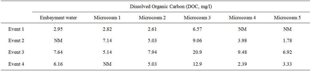
Table 4. Dissolved organic carbon in embayment water and in microcosm samples at the end of each event.
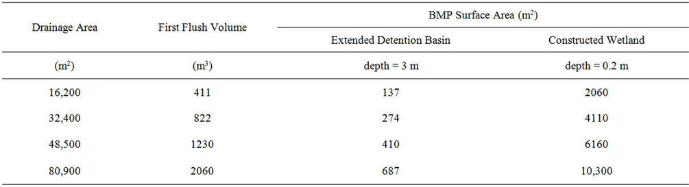
Table 5. Expected BMP surface areas required based on a first flush stormwater volume from a drainage area.
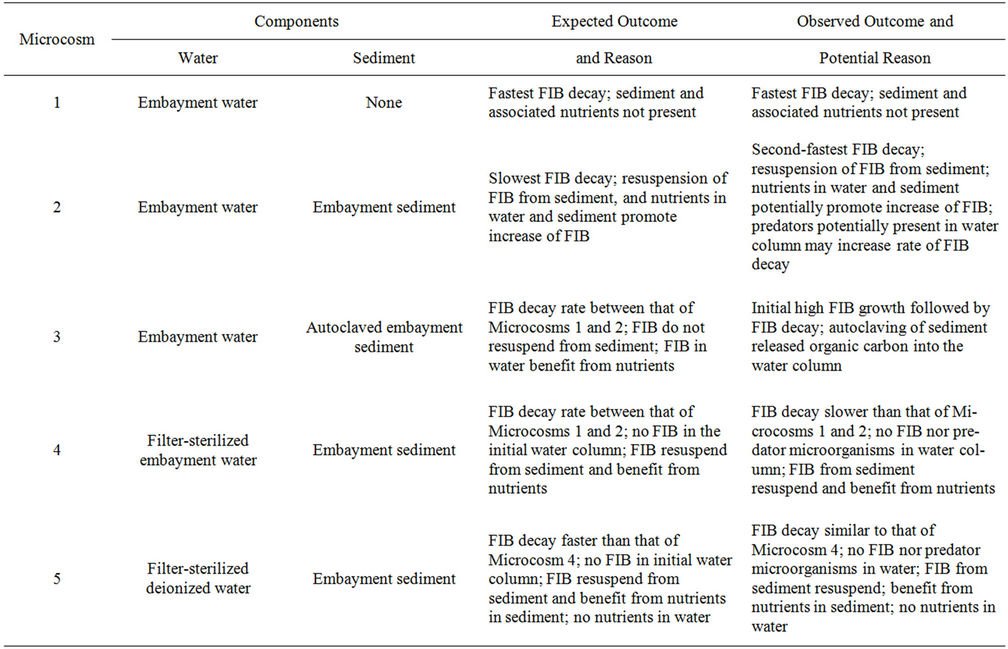
Table 6. Expected and observed outcomes of microcosm events.
The results of the FIB decay rates in the microcosms relate to stormwater BMPs in that the assumptions in this study were in agreement with the conclusions from the International Stormwater BMP Database [23] as well as the US Environmental Protection Agency (USEPA) report on retention ponds and constructed wetlands [24]. Detention ponds and constructed wetlands have consistently lacked effectiveness in reducing FIB in stormwater runoff. As the calculations of this study have shown, the time required to reduce the FIB in the waters can be as much as 107 hours, which is not a reasonable amount of time to contain stormwater runoff. For example, Davis and McCuen [25] report residence times of less than 24 hours for extended detention basins and constructed wetlands. According to USEPA [24], the presence of sediments is likely the cause of BMP failure to lower FIB levels. The results from the controlled laboratory experiments, and specifically Microcosms 1 and 2, are consistent with this conclusion as well, especially with the assumption that FIB do not settle to the bottom because of turbulence in the water.
While it is no surprise that FIB persist longer in the water column when sediments are present [26,27], we can conclude that nutrients originating from sediment are significant for FIB longevity. Because nutrients in the form of organic carbon released from sediment did increase survival of FIB (in the case of Microcosm 3), it can be concluded that sediment-associated nutrients cannot be ignored, though further studies would be necessary to determine what form of organic carbon was released in autoclaving. This finding is consistent with microbiology literature. For example, one study reports that E. coli in lake water considerably increased within 24 hours of inoculation into sterile, autoclaved sand and mud, followed by a 2 to 3 day stationary period, then a decrease [28]. Although autoclaving of sediment is not field-applicable, there is a confirmation of the literature [29] that high levels of assimilable organic carbon (AOC) in the water column can significantly alter the decay rate constant for FIB, showing that organic carbon content should be considered in determining modeling parameters and in the effectiveness of stormwater BMPs. An example of the latter is a stormwater treatment wetland with plants in various states of decay. Decaying material can release dissolved organic carbon into the water column, potentially reducing the treatment effectiveness of the wetland for FIB. These results demonstrate that, to fully troubleshoot water quality exceedances for FIB in BMPs, analyses of sediment, organic carbon, and water column depth should be conducted. Finally, the net decay rates calculated are key parameters for determining the required detention time for FIB-laden stormwater in detention basins, constructed wetlands, and other structural BMPs requiring storage of water.
5. Acknowledgements
This study was funded by a grant from the U.S. Geological Survey through the Mississippi Water Resources Research Institute (06HQGR0094, subaward 080600- 330920-01) with matching funds from the University of Mississippi (UM). We thank student Keah Y. Lim for assistance in the field and laboratory, Sam Testa and Doug Shields of the USDA National Sedimentation Laboratory in Oxford, MS, Cliff Ochs of the Department of Biology at UM, and the UM Department of Chemical Engineering.
REFERENCES
- J. M. Colford, T. J. Wade, K. C. Schiff, C. C. Wright, J. F. Griffith, S. K. Sandhu, S. Burns, M. D. Sobsey, G. Lovelace and S. B. Weisberg, “Water Quality Indicators and the Risk of Illness at Beaches with Nonpoint Sources of Fecal Contamination,” Epidemiology, Vol. 18, 2007, pp. 27-35.
- D. Mardon and D. Stretch, “Comparative Assessment of Water Quality at Durban Beaches according to Local and International Guidelines,” Water SA, Vol. 30, No. 3, 2004, pp. 317-324. Hdoi:10.4314/wsa.v30i3.5079
- USEPA, “National Summary of Impaired Waters and TMDL Information,” 2012. http://iaspub.epa.gov/waters10/attains_nation_cy.control?p_report_type=T
- C. Q. Surbeck, S. C. Jiang, J. H. Ahn and S. B. Grant, “Flow Fingerprinting Fecal Pollution and Suspended Solids in Stormwater Runoff from an Urban Coastal Watershed,” Environmental Science & Technology, Vol. 40, No. 14, 2006, pp. 4435-4441. Hdoi:10.1021/es060701h
- T. M. Petersen, H. S. Rifai, M. Suarez and A. R. Stein, “Bacteria Loads from Point and Nonpoint Sources in an Urban Watershed,” ASCE Journal of Environmental Engineering, Vol. 131, No. 10, 2005, pp. 1414-1425. Hdoi:10.1061/(ASCE)0733-9372(2005)131:10(1414)
- H. Li and A. P. Davis, “Water Quality Improvement through Reductions of Pollutant Loads Using Bioretention,” ASCE Journal of Environmental Engineering, Vol. 135, No. 8, 2009, pp. 567-576. Hdoi:10.1061/(ASCE)EE.1943-7870.0000026
- J. M. Hathaway, W. F. Hunt and S. Jadlocki, “Indicator Bacteria Removal in Storm-Water Best Management Practices in Charlotte, North Carolina,” ASCE Journal of Environmental Engineering, Vol. 135, No. 12, 2009, pp. 1275-1285. Hdoi:10.1061/(ASCE)EE.1943-7870.0000107
- B. M. Wadzuk, M. Rea, G. Woodruff, K. Flynn and R. G. Traver, “Water-Quality Performance of a Constructed Stormwater Wetland for All Flow Conditions,” Journal of the American Water Resources Association, Vol. 46, No. 2, 2010, pp. 385-394. Hdoi:10.1111/j.1752-1688.2009.00408.x
- E. M. Smith and Y. T. Prairie, “Bacterial Metabolism and Growth Efficiency in Lakes: The Importance of Phosphorus Availability,” Limnology and Oceanography, Vol. 49, No. 1, 2004, pp. 137-147. Hdoi:10.4319/lo.2004.49.1.0137
- C. Q. Surbeck, S. C. Jiang and S. B. Grant, “Ecological Control of Fecal Indicator Bacteria in an Urban Stream,” Environmental Science & Technology, Vol. 44, No. 2, 2010, pp. 631-637. Hdoi:10.1021/es903496m
- H. C. Jeng, A. J. England and H. B. Bradford, “Indicator Organisms Associated with Stormwater Suspended Particles and Estuarine Sediment,” Journal of Environmental Science and Health, Vol. 40, No. 4, 2005, pp. 779-771. Hdoi:10.1081/ESE-200048264
- C. H. Bolster, J. M. Bromley and S. H. Jones, “Recovery of Chlorine-Exposed Escherichia coli in Estuarine Microcosms,” Environmental Science & Technology, Vol. 39, No. 9, 2005, pp. 3083-3089. Hdoi:10.1021/es048643s
- D. L. Craig, H. J. Fallowfield and N. J. Cromar, “Use of Microcosms to Determine the Persistence of Escherichia coli in Recreational Coastal Water and Sediment and Validation with in Situ Measurements,” Journal of Applied Bacteriology, Vol. 96, No. 5, 2004, pp. 922-930. Hdoi:10.1111/j.1365-2672.2004.02243.x
- R. L. Smith, “The Resilience of Bottomland Hardwood Wetlands Soils Following Timber Harvest,” M.S. Thesis, University of Mississippi, Oxford, 1997.
- Soil Survey Division Staff, “Soil Survey Manual,” Handbook 18, US Department of Agriculture, Soil Conservation Service, 1993.
- D. L. Craig, H. J. Fallowfield and N. J. Cromar, “Enumeration of Faecal Coliforms from Recreational Coastal Sites: Evaluation of Techniques for the Separation of Bacteria from Sediments,” Journal of Applied Microbiology, Vol. 93, No. 4, 2002, pp. 557-565. Hdoi:10.1046/j.1365-2672.2002.01730.x
- Y. Jeong, S. B. Grant, S. Ritter, A. Pednekar, L. Candelaria and C. Winant, “Identifying Pollutant Sources in Tidally Mixed Systems: Case Study of Fecal Indicator Bacteria from Marinas in Newport Bay, Southern California,” Environmental Science & Technology, Vol. 39, No. 23, 2005, pp. 9083-9093. Hdoi:10.1021/es0482684
- A. D. Eaton, L. S. Clesceri, E. W. Rice and A. E. Greenbert, “Standard Methods for the Examination of Water and Wastewater,” American Public Health Association, American Water Works Association, Water Environment Federation, Washington DC, 2005.
- D. W. Nelson and L. E. Sommers, “Total carbon, organic carbon, and organic matter,” In: A. L. Page, et al., Eds., Methods of Soil Analysis Part 2, American Society of Agronomy, Madison, 1996, pp. 961-1010.
- USEPA, “Total Maximum Daily Loads with Stormwater Sources: A Summary of 17 TMDLs, July 2007 EPA 841- R-07-002,” National Center of Environmental Publications, Washington DC, 2007.
- USEPA, “Ambient Water Quality Criteria for Bacteria— 1986. EPA 440-5-84-002,” National Center of Environmental Publications, Washington DC, 1986.
- S. C. Chapra, “Surface Water-Quality Modeling,” WCB McGraw-Hill, Boston, 1997.
- Wright Water Engineers Inc. and Geosyntec Consultants, “International Stormwater BMP Database, Pollutant Category Summary: Fecal Indicator Bacteria,” 2010. www.bmpdatabase.org
- S. D. Struck, A. Selvakumar and M. Borst, “Performance of Stormwater Retention Ponds and Constructed Wetlands in Reducing Microbial Concentrations EPA 600-R- 06-102,” National Risk Management Research Laboratory, Urban Watershed Management Branch, Edison, NJ, 2006.
- A. P. Davis and R. H. McCuen, “Stormwater Management for Smart Growth,” Springer, New York, 2005.
- H. M. Solo-Gabriele, M. A. Wolfert, T. R. Desmarais and C. J. Palmer, “Sources of Escherichia coli in a Coastal Subtropical Environment,” Applied and Environmental Microbiology, Vol. 66, 2000, pp. 230-237.
- R. Fujioka, C. Sian-Denton, M. Borja, J. Castro and K. Morphew, “Soil: The Environmental Sources of E. coli and Enterococci in Guam’s Streams,” Journal of Applied Microbiology Symposium Supplement, Vol. 85, 1999, pp. 83S-89S.
- P. La Liberte and D. J. Grimes, “Survival of Escherichia coli in Lake Bottom Sediment,” Applied and Environmental Microbiology, Vol. 43, No. 3, 1982, pp. 623-628.
- M. Vital, D. Stucki, T. Egli and F. Hammes, “Evaluating the Growth Potential of Pathogenic Bacteria in Water,” Applied and Environmental Microbiology, Vol. 76, No. 19, 2010, pp. 6477-6484. Hdoi:10.1128/AEM.00794-10
NOTES
*Corresponding author.