Smart Grid and Renewable Energy
Vol. 4 No. 1 (2013) , Article ID: 28114 , 10 pages DOI:10.4236/sgre.2013.41001
Wind Turbine Power Output Assessment in Built Environment
![]()
1Division of Mechanical Engineering, Graduate School of Engineering, Mie University, Tsu, Japan; 2School of Energy & Resources, University of College London, Adelaide, Australia.
Email: *nisimura@mach.mie-u.ac.jp
Received September 3rd, 2012; revised October 3rd, 2012; accepted October 10th, 2012
Keywords: Wind Turbine; Wind Energy in Built Environment; Wind Velocity Distribution across Buildings; Urban Wind Resource Assessment
ABSTRACT
In future planning of the city, it is very important to consider the proper intelligent integration of renewable energy sources into the built environment for developing smart cities. Analysis of the wind velocity profile in the built environment is very important for finding out the energy content in the wind and also to analyze the performance of wind turbines in the built environment. In this study, building topologies of smart city are investigated for finding out the wind velocity profile and the wind turbine power output in the built environment. The wind velocity distribution across buildings is numerically simulated by using commercial CFD (Computational Fluid Dynamics) software CFD-ACE+. Wind turbine power output is estimated by using the power curve of real commercial wind turbine and wind velocity distribution simulated by CFD software. It has been observed that the wind is accelerated in the intervening space between the buildings irrespective of distance between the walls of adjacent buildings under the condition, which are investigated in this study. The wind is accelerated across buildings, and is reduced rapidly after blowing through buildings, and recovered gradually. Since the wind is accelerated in the intervening space between buildings and reduced in the area at the back of buildings, a wind turbine should be installed at the area at the back of the buildings and located on center between the buildings. In this work, it is observed that size dimensions and layout of the building are effective in realizing a smart city for utilizing renewable energy such as wind turbine in the built environment.
1. Introduction
Since a fossil fuel reserve is limited and a global warming by greenhouse gas like CO2 is a worldwide problem, environment friendly energy sources are requested to fulfill the growing energy demand and also to replace the fossil fuelled existing power plants. Renewable energy sources such as wind, photovoltaic, solar thermal, geothermal and bio-energy draw attention from the world as an alternative environment friendly energy sources. Since the energy density of these described renewable energy sources is low and they are also nature dependent. It is very important to develop proper strategies to integrate these renewable energy sources into the network for buffering their intermittency and also to improve the power system stability with higher penetration of renewable energy sources. The smart grid is an effective way to integrate renewable energy sources into the existing energy system network [1-6]. A future smart grid power system network will serve as a dynamic network for multi-directional energy flows, linking widely distributed small capacity renewable energy systems at consumer level (distribution network) and centralized higher-capacity power generators, facilitating active participation of customer choice for energy production/source and demand management, and also providing real-time information on the performance and optimal operation of the power system network [3]. A major evolutionary step in the grid’s design, planning, and operation is needed using new design concepts and technologies which can be integrated into the power system network. Smart grid power system network configuration will provide clear economic and environmental benefits, and will contribute significantly to achieving a wide range of government objectives e.g. sustainable development, energy supply security, diversity and reliability etc. A smart grid research and technology development, demonstration and deployment effort has to harmonize with expansion of the power system infrastructure, the information and communications infrastructure with modern actuators/ sensors, and integration of new monitoring and control applications [3].
In Japan, some demonstration projects of smart city are under contemplation [7]. In China, Tianjin City is being rebuilt as ecological city by project in collaboration with Singapore company [8]. This trend will continue and many cities will be rebuilt as smart city in near future. In the built environment, it will be difficult to integrate the renewable energy sources and distributed generators as the existing building infrastructure are not designed to integrate renewable energy sources into the network. In future planning of the city, it is very important to consider in the smart city design proper intelligent integration of renewable energy sources into the built environment.
In this study, building topologies of smart city are investigated for finding out the wind velocity profile in the built environment. Analysis of the wind velocity profile in the built environment is very important for finding out the energy content in the wind and also to analyze the performance of wind turbines in the built environment. The micro/mini-scale wind turbines are emerging as building integrated renewable energy technology due to advances in aerodynamic design, electric generators, power condition devices, increasing energy prices and the financial incentives provided by the government. The output from these built environment wind turbines are affected by the shear and shadow effects of the wind velocity profile distribution in the built environment. The generalized quantification of built environment wind turbines is uncertain. In the first phase, this study focuses on the size and layout of buildings in the smart city. In the built environment, the wind velocity distribution is mainly influenced by the dimensions, design and layout of the buildings. The analysis of the wind velocity profile in the built environment is very important to find the energy content in the wind. It will help in finding the effective wind energy input on the wind turbine and its output.
The concept diagram of this study has been illustrated in Figure 1. The wind velocity profile changes in the built environment and accelerated by blowing through the buildings. Therefore the resulting wind velocity becomes more than the input wind before the inbuilt environment. It has been observed by the authors that in most of the studies the normal wind velocity profile has been considered for finding the performance of the wind turbines in the built environment. Therefore it is necessary to analyze the wind velocity profile in the built environment for analyzing the performance of the building integrated wind turbines taking into account the building profiles and their layouts.
The main objective of this study is to estimate the generated power output of wind turbine for wind velocity variations in the built environment by taking into account the building profiles and their layouts. Also, the effective design of building layouts are analyzed for obtaining the higher output from the building integrated wind turbines. As far as the authors’ survey literatures, there is no study that analyzes the wind velocity distribution around building to obtain the higher output of wind turbine. In this study, the estimation of the power output of the building integrated wind turbine is analyzed by using the wind velocity distribution across the buildings. The wind velocity distribution across the buildings is developed/ simulated through a CFD (Computational Fluid Dynamics) software. The output power of the wind turbine is estimated by using the power curve of real commercial wind turbine and the wind velocity distribution around buildings.
2. Power Output Estimation of Building Integrated Wind Turbine
2.1. Simulation of Wind Velocity Distribution around the Buildings
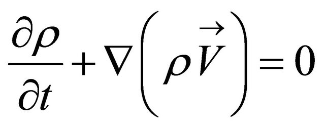
In this study, a commercial CFD software CFD-ACE+ (WAVE FRONT) is adopted for numerical simulation of wind velocity distribution. This CFD software has many simulation code/tools for solving the fluid dynamics. The validation of the simulation procedure of this CFD software has been well established [9-14]. The standard  model is adopted in this study. In the CFD software, the continuity equation is given by [15,16]:
 (1)
(1)
where  is density,
  is time and
  is velocity vector.
The momentum equation is given by [15,16]:
 (2)
(2)
 (3)
(3)
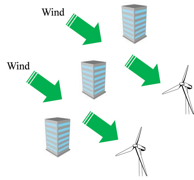
Figure 1. Concept diagram of this study.
where  is velocity at
  component of coordinate system,
 ![]() is pressure,
is pressure,  is effective viscosity coefficient,
 ![]() is viscosity coefficient and
is viscosity coefficient and  is eddy viscosity coefficient.
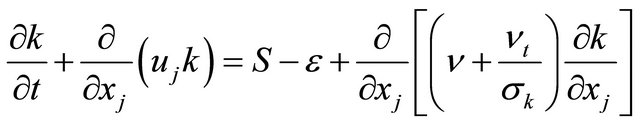
In the CFD software, the standard  model is given by [15,16]:
 (4)
(4)
 (5)
(5)
 (6)
(6)
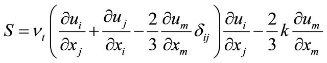 (7)
(7)
where  is turbulent energy,
 ![]() is dissipation rate, δij is Kronecker delta,
is dissipation rate, δij is Kronecker delta,  is 0.09,
  is 1.44,
  is 1.92,
  is 1.0,
  is 1.3. Regarding
  which represent components of coordinate system,
 . Regarding
  which represent velocities,
  ,
,  ,
, .
.  is the velocity component of coordinate system,
  respectively.
To validate the simulation code in the CFD software, the simulation result on wind velocity distribution around a block is compared with the reference [17], which simulates the wind velocity distribution around a cubic block by standard  model. Figure 2 shows the model simulated by the study [17], which is used as validation in this work. The cubic block is 0.12 m on a side. Representative length of this model
  is set at 0.12 m.
Table 1 lists the simulation condition of the reference [17], which is adopted for validation of this study. Most of the boundary conditions of this study are used from the reference [17]. The wind velocity distribution at inlet of the model is developed by using the equation given in Table 1 and Figure 3. Outlet of the model is going without any disturbance of the built environment. The top layer of the model has been considered free (without any disturbance) though the reference sets slip condition. The slip on side wall of block is set by the following equation:
 (8)
(8)
where  is the mixing length, 0.41 is Karman coefficient,
  is distance from wall of block.
After validation of the simulation procedure, the wind velocity distribution around the buildings, which is proposed in this study, is simulated. Figure 4 shows the

Figure 2. Model of simulation for validation.
Table 1. Simulation condition of reference.
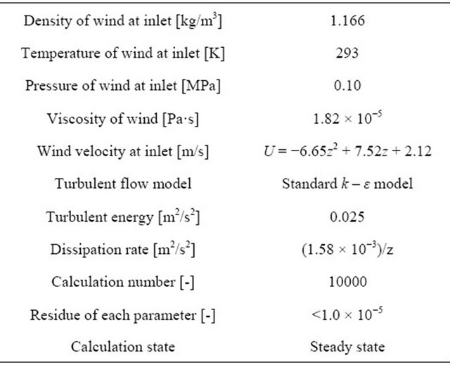
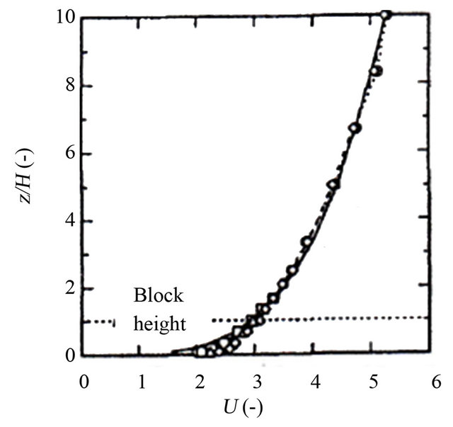
Figure 3. Wind velocity distribution condition at inlet for validation.
building model which indicates the case of building distance of 20 m. Building dimensions are 20 m × 20 m × 40 m. The representative length of this model ![]() is set at 20 m. As shown in Figure 1, several numbers of buildings are required to accelerate the wind by blowing through the combination of buildings. This study sets three buildings and two wind turbines as basic combination. If the optimum condition can be obtained for accelerating the wind, then the high wind power generation will be available by doing the proper layout of the buildings and the wind turbines. As shown in Figure 4, the wind turbine is not set in the model, resulting that the impact of wind turbine on downstream wind velocity distribution is not considered in this simulation work. Both sides of model have a slope which assumes a hill zone. This study assumes that the buildings are located at the bottom of the hill zone, and the wind blows through the hill zone. The main objective of this study is to suggest a proper location, where the wind velocity can be accelerated.
is set at 20 m. As shown in Figure 1, several numbers of buildings are required to accelerate the wind by blowing through the combination of buildings. This study sets three buildings and two wind turbines as basic combination. If the optimum condition can be obtained for accelerating the wind, then the high wind power generation will be available by doing the proper layout of the buildings and the wind turbines. As shown in Figure 4, the wind turbine is not set in the model, resulting that the impact of wind turbine on downstream wind velocity distribution is not considered in this simulation work. Both sides of model have a slope which assumes a hill zone. This study assumes that the buildings are located at the bottom of the hill zone, and the wind blows through the hill zone. The main objective of this study is to suggest a proper location, where the wind velocity can be accelerated.
Table 2 lists the simulation condition in this study. Wind velocity at inlet of the model is set by the following equation:
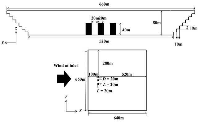
Figure 4. Model of simulation for wind power generation.
Table 2. Simulation condition of this study.
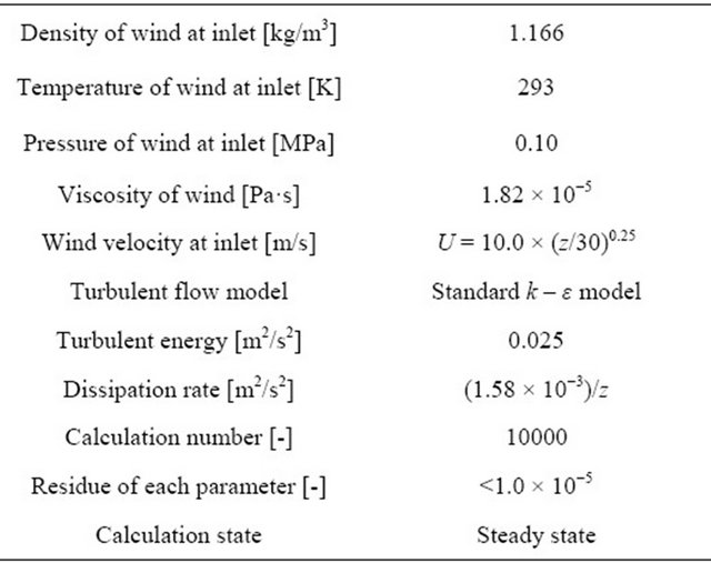
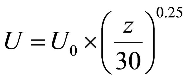 (9)
(9)
where  = 10.0 m/s which is the rated wind velocity of AEOLOS wind turbine of 50 kW class (AEOLOS: wind turbine manufacturer) [18].
In Equation (9), wind velocity is 10.0 m/s at the height of 30 m which is the hub height of the wind turbine when the wind reaches to the building.
Most of the boundary conditions in this simulation, excluding wind velocity at inlet of the model, follow the boundary conditions of simulation validation as shown in Table 1.
2.2. Concept of Building Size Setting
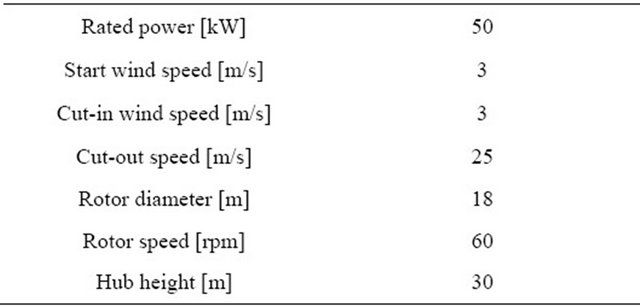
This study assumes that building in the model is multi storied apartment. According to the statistics data collected by ministry of internal affairs and communications in Japan [19], the average floor space of dwelling of Japan is about 100 m2 per a household. The height of one floor is assumed as 4 m. Assuming that four households stay per floor, the floor space is 400 m2. In the simulation of this study, the width and depth of building is set at 20 m and 20 m, respectively. The height of building should be set over the height of wind turbine if we request an accelerated wind by blowing through buildings. In this study, the real commercial wind turbine is adopted for estimating the power generated by wind velocity distribution. AEOLOS wind turbine of 50 kW class [18] is adopted in this study.
Table 3 lists the specification of AEOLOS wind turbine of 50 kW class. The hub height and rotor radius of this turbine is 30 m and 9 m, respectively, resulting that the height of building is set at 40 m.
2.3. Estimation of Power Generated by Wind Turbine
The wind at the area at the back of buildings is thought to be available for power generation by wind turbine, since the wind would be accelerated by blowing through buildings. The area at the back of buildings of 20 m, 30 m, and 40 m is assumed as the installation point of wind
Table 3. Specification of wind turbine.
turbine. The wind velocity for calculating the power generated by wind turbine is obtained on 1049 points located in the area where the rotor of wind turbine rotates, that is, the swept rotor area. The wind velocity at each point on the swept rotor area is the averaged velocity in the local area of 0.5 m × 0.5 m. By using the wind velocity distribution of this local wind velocity, the wind energy can be calculated. Average wind velocity is estimated by using the following equation:
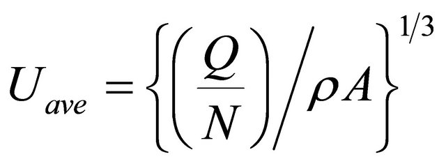 (10)
(10)
where  is the average wind velocity,
  is the wind energy calculated for area where rotor of wind turbine rotates,
  is points for calculating wind velocity distribution (= 1049 points),
  is the area where rotor of wind turbine rotates.
  is summation of wind energy on each point for calculating wind velocity distribution. Wind energy at each point on the swept rotor area is calculated by the following equation:
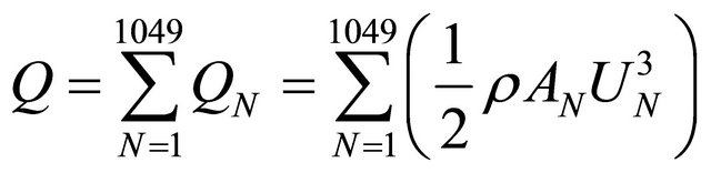 (11)
(11)
where  is the wind energy at each point,
  is the area of each point which is equal to 0.5 m × 0.5 m,
  is the wind velocity at each point for calculating wind energy. In estimation of power generation, the wind energy at the point whose wind velocity is below 3 m/s is omitted since the cut-in wind speed of AEOLOS wind turbine of 50 kW class is 3 m/s.
The power curve of AEOLOS wind turbine of 50 kW is shown in Figure 5. The authors derive the empirical equation from the data of power curve, which is provided by AEOLOS. Figure 5 indicates the relationship between wind and power, resulting that the power generated by this wind turbine can be estimated by using the power curve.
The power curve which is adopted in this study is as follows:
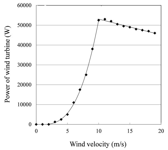
Figure 5. Power curve of wind turbine.
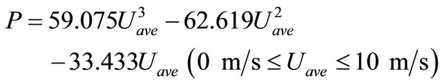 (11)
(11)
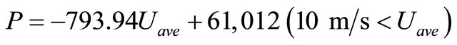 (12)
(12)
where  is a power of wind turbine.
3. Results and Discussion
3.1. Validation of Numerical Simulation Procedure
To validate the performance of the present numerical simulation procedure, the wind velocity distribution around the block is compared with the result of reference [17]. Figure 6 shows the comparison of contour of wind velocity distribution around block on ![]() cross section between this study and reference. In this figure, the wind velocity distribution to
cross section between this study and reference. In this figure, the wind velocity distribution to ![]() direction at
direction at  is shown. Figure 7 shows the comparison of contour of wind velocity distribution around block on
  cross
cross

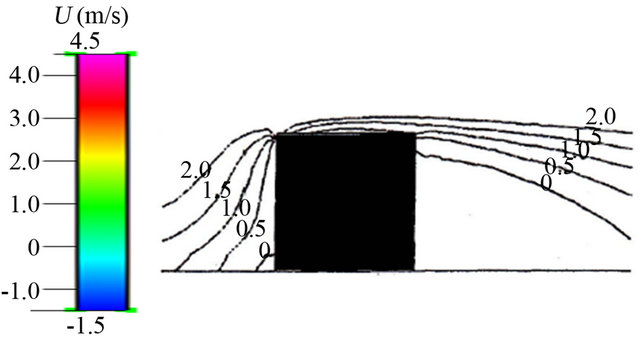
Figure 6. Comparison of contour of wind velocity distribution around block at y/H = 0 on x – z cross section between this study and reference (left: this study, right: reference).


Figure 7. Comparison of contour of wind velocity distribution around block at z/H = 0.5 on x – y cross section between this study and reference (left: this study, right: reference).
section between this study and reference. In this figure, the wind velocity distribution to ![]() direction at
direction at  is shown.
According to Figures 6 and 7, the results obtained by present numerical simulation procedure are in good agreement with the established results in reference [17]. The standard  model can simulate the wind velocity distribution around block well.
Figures 8 and 9 show the comparison of wind velocity distribution around block on ![]() cross section between this study and reference [17]. Figure 8 shows the change in wind velocity distribution to
cross section between this study and reference [17]. Figure 8 shows the change in wind velocity distribution to ![]() direction at
direction at , while Figure 9 shows the change in wind velocity distribution to x direction at
 . In these figures, the wind velocity distribution at
  is shown.
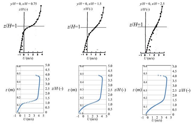
Figure 8. Comparison of wind velocity distribution at y/H = 0 around block on x – z cross section between this study and reference (top: reference, bottom: this study).
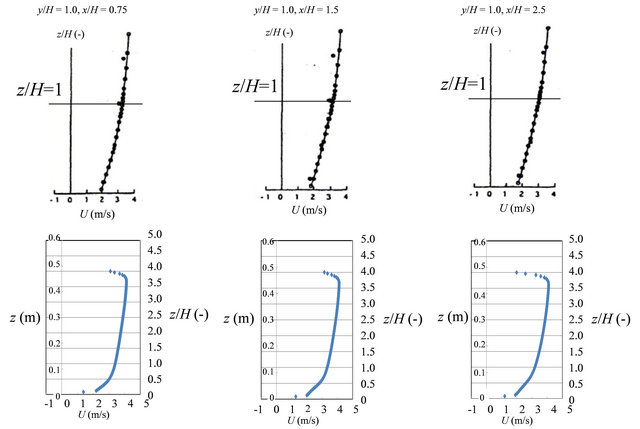
Figure 9. Comparison of velocity distribution at y/H = 1.0 around block on x – z cross section between this study and reference (top: reference, bottom: this study).
According to Figures 8 and 9, the results obtained by present numerical simulation procedure are in good agreement with the established results in reference. The wind velocity distribution near the top of the model for this study is a little different from the reference, and it is due to the difference of the boundary condition as mentioned above.
However, this difference near the top of the model is not important in this study, since this work analyzes the wind velocity distribution around the building of 40 m height which is equal to  in the validation. Since the good agreement is obtained around
  in the validation, therefore it can be said that the availability of numerical simulation procedure in this study is proved.
3.2. Simulation of Wind Velocity Distribution around Buildings and Estimation of Power Generated by Wind Turbine
Figure 10 shows contours of wind velocity distribution around buildings at  which is hub height of wind turbine on
  cross section. In this figure, the effect of distance between the buildings, which is changed by 10 m, 20 m, 40 m and 60 m
( ), is investigated (where
  represents the distance between walls of adjacent buildings). In this model,
  and
and  is located at the center of middle building among three buildings irrespective of
 . In this figure, black lines mean the separation lines which distinguish the different calculation domain in the model used for numerical simulation in this study. From this figure, it is seen that the wind is accelerated in the intervening space between buildings irrespective of
  under the investigating condition of this study, since some wind is over the initial wind velocity
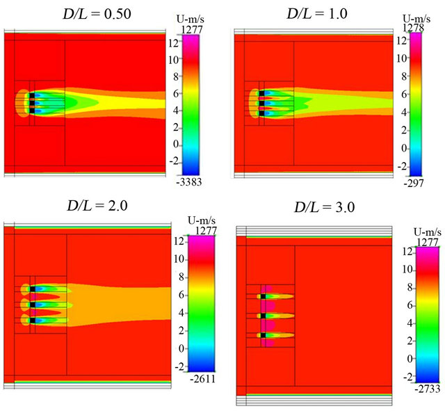
Figure 10. Contour of wind velocity distribution around buildings at z = 30 m on x – y cross section.
of  of 10 m/s. In addition, the area where the accelerated wind is obtained is wider towards y direction with increasing
 . To obtain good wind velocity distribution, a wind turbine should be installed at the area at the back of buildings and located on center between two buildings.
Figure 11 shows comparison of wind velocity distribution to x direction at  on
on ![]() cross section. The effect of
cross section. The effect of , which is changed by
  , on wind velocity distribution is investigated. In this figure,
  is divided by
  which is the wind velocity at the inlet of model at
 , i.e., U = 10 m/s. The wind velocity distribution to x direction for
  is shown at y = 15 m, 20 m, 30 m and 40 m, respectively, which is the wind velocity distribution at the center between two buildings for each D. According to Figure 11, the accelerated wind, i.e.,
  is over unity, is seen around buildings which is around x = 0 m, i.e., from x = −10 m to x = 40 m for
 . Then, it can suggest that wind turbine sets at this area to obtain good wind velocity distribution.
In addition, the wind velocity drops rapidly after blowing through buildings, and recovered gradually. Though the highest wind velocity is obtained for D/L = 1.0, the wind velocity drops rapidly after blowing through buildings. The wind velocity at the area at the back of buildings is recovered faster with increasing D except for D/L = 0.50. Regarding D/L = 0.50, most of wind cannot blow through buildings since the distance between buildings is narrow. The wind blows keeping from space between buildings, resulting that the wind velocity in the area at back of buildings is slow compared to other D. Since most of wind blows through surrounding of buildings, the wind velocity at area at the back of buildings which have enough distance from buildings are recovered rapidly by wind energy supply from surrounding wind.
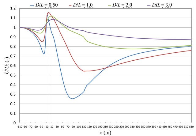
Figure 11. Comparison of wind velocity distribution to x direction at z = 30 m on x - z cross section.
Figures 12-15 show the contour of the wind velocity distribution around buildings at x = 20 m, 30 m and 40 m ( = 1.0, 1.5 and 2.0) on
  cross section for
  = 0.50, 1.0, 2.0 and 3.0, respectively. In these figures, black cross line represents the rotor diameter of wind turbine, and black rectangular lines represent the location of buildings. From these figures, the higher wind velocity is obtained for smaller
 , that is, near the building as described above. However, the wind velocity drop toward x direction is relatively small excluding
  = 0.50 if x is within 40 m (
 ). In addition, it is known that the wind is accelerated in the intervening space between buildings and reduced in the area at the back of buildings irrespective of
  and
and  under the investigating condition in this study. Therefore, a wind turbine should be installed at the area at the back of buildings and located on center between the two buildings. Moreover, when
  is narrow such as
  = 0.50 and 1.0, it can be seen that slow wind velocity is in the area where the rotor of wind turbine rotates. Hence, it reveals that the optimum buildings distance exists for obtaining good wind velocity distribution.
Figure 12. Contour of wind velocity distribution at the area at the back of buildings of x/L = 1.0, 1.5 and 2.0 on y – z cross section for D/L = 0.50.

Figure 13. Contour of wind velocity distribution at the area at the back of buildings of x/L = 1.0, 1.5 and 2.0 on y – z cross section for D/L = 1.0.
Figure 14. Contour of wind velocity distribution at the area at the back of buildings of x/L = 1.0, 1.5 and 2.0 on y – z cross section for D/L = 2.0.
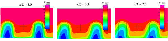
Figure 15. Contour of wind velocity distribution at the area at the back of buildings of x/L = 1.0, 1.5 and 2.0 on y – z cross section for D/L = 3.0.
According to Figures 12-15, Tables 4-7 list ,
,  and
and  at
at  = 1.0, 1.5 and 2.0 for
  = 0.50, 1.0, 2.0 and 3.0, respectively. It is observed from Tables 4 and 5 that
  and
and  are small, when D is narrow such as
  = 0.50 and 1.0. On the other hand, high
  and
and  are obtained at
  = 2.0 and 3.0 and they are shown in Tables 6 and 7.
Though  and
and  increase with increasing
 , the difference of
  and
and  between
  = 2.0 and
  = 3.0 is a small. Hence, it reveals that the optimum
Table 4. Comparison of Q, Uave and P among different x/L for D/L = 0.50.
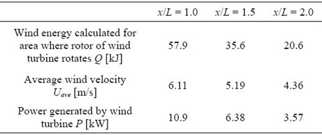
Table 5. Comparison of Q, Uave and P among different x/L for D/L = 1.0.
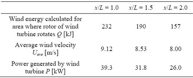
Table 6. Comparison of Q, Uave and P among different x/L for D/L = 2.0.
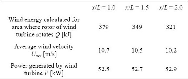
Table 7. Comparison of Q, Uave and P among different x/L for D/L = 3.0.
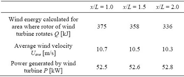
buildings distance exists for obtaining good wind velocity distribution. Since  is over
  for
for  = 2.0 and 3.0, it can be said that the accelerated wind is obtained by wind blowing through buildings. Finally, it is clarified that size, dimensions and layout of building are effective to realize a smart city for utilizing renewable energy in the built environment.
4. Conclusions
In future planning of the city, it is very important to consider the proper intelligent integration of renewable energy sources into the built environment for developing smart cities. In this study, building topologies of smart city are investigated for finding out the wind velocity profile in the built environment. Analysis of the wind velocity profile in the built environment is very important for finding out the energy content in the wind and also to analyze the performance of wind turbines in the built environment. The output from these built environment wind turbines are affected by the shear and shadow effects of the wind velocity profile distribution in the built environment. The wind velocity distribution across the buildings is simulated by CFD software. Wind turbine power output is estimated by using the power curve of real commercial wind turbine and wind velocity distribution simulated by CFD software. As a result, the following conclusions have been obtained from this study.
1) The results obtained by using the numerical simulation procedure are in good agreement with the established results in reference [17]. The numerical simulation procedure of this study is suitable for simulating the wind velocity distribution across the buildings.
2) The wind is accelerated in the intervening space between the buildings irrespective of  under the investigating condition of this study.
3) The accelerated wind is obtained across buildings, and wind velocity drops rapidly after blowing through buildings, and recovered gradually. When the back distance from building is within 40 m ( ), the wind is accelerated and wind velocity drop toward x direction is relatively small.
4) The wind is accelerated in the intervening space between the buildings and reduced in the area at the back of buildings irrespective of  and
and  under the investigating condition of this study. A wind turbine should be installed at the area at the back of buildings and located on center between two buildings.
5) There is an optimum  for obtaining good wind velocity distribution, in other words, high
  and
and .
.
REFERENCES
- M. Liserre, T. Sauter and J. Y. Hung, “Future Energy Systems,” IEEE Industrial Electronics Magazine, 2010, pp. 18-37.
- L. F. Ochoa and G. P. Harrison, “Minimizing Energy Losses: Optimal Accommodation and Smart Operation of Renewable Distributed Generation,” IEEE Transactions on Power System, Vol. 26, No. 1, 2011, pp. 198-205. doi:10.1109/TPWRS.2010.2049036
- M. Kolhe, “Smart Grid: Charting a New Energy Future: Research, Development and Demonstration,” The Electricity Journal, Vol. 25, No. 2, 20112, pp. 88-93.
- M. Wissner, “The Smart Grid—A Saucerful of Secrets?” Applied Energy, Vol. 88, No. 7, 2011, pp. 2509-2518. doi:10.1016/j.apenergy.2011.01.042
- M. Kolhe, K. Agbossou, J. Hamelin and T. K. Bose, “Analytical Model for Predicting the Performance of Photovoltaic Array Coupled with a Wind Turbine in a Stand-Alone Renewable Energy System Based on Hydrogen,” Renewable Energy, Vol. 28, No. 5, 2003, pp. 727-742. doi:10.1016/S0960-1481(02)00107-6
- T. Vijayapriya and D. P. Kothari, “Smart Grid: An OverView,” Smart Grid and Renewable Energy, Vol. 2, No. 2, 2011, pp. 305-311. doi:10.4236/sgre.2011.24035
- “Ministry of Economy, Trade and Industry in Japan,” 2012. http://www.meti.go.jp/english/index.html
- “Smart Grid Demonstration Project in Sino-Singapore Tianjin Eco-City,” http://www.sgiclearinghouse.org/Asia?q=node/2594&lb=1
- C. Y. Wen, A. S. Yang, L. Y. Tseng and W. T. Tsai, “Flow Analysis of a Ribbed Helix Lip Seal with Consideration of Fluid-Structure Interaction,” Computers & Fluids, Vol. 40, No. 1, 2011, pp. 324-332. doi:10.1016/j.compfluid.2010.10.005
- H. H. Caicedo, M. Hernandez, C. P. Fall and D. T. Eddington, “Multiphysics Simulation of a Microfluidic Perfusion Chamber for Brain Slice Physiology,” Biomed Microdevices, Vol. 12, No. 5, 2010, pp. 761-767. doi:10.1007/s10544-010-9430-5
- C. Xing, M. J. Braun and H. Li, “Damping and Added Mass Coefficients for a Squeeze Film Damper Using the Full 3-D Navier Stokes Equation,” Tribology International, Vol. 43, No. 3, 2010, pp. 654-666.
- G. Demirkaya, C. W. Soh and O. J. Ilegbusi, “Direct Solution of Navier-Stokes Equations by Radial Basis Functions,” Applied Mathematical Modeling, Vol. 32, No. 9, 2008, pp. 1848-1858.
- T. Glatzel, C. Litterst, C. Cupelli, T. Lindrmann, C. Moosmann, R. Niekrawietz, W. Streule, R. Zengerle and P. Koltay, “Computational Fluid Dynamics (CFD) Software Tools for Microfluidic Applications—A Case Study,” Computers & Fluids, Vol. 37, No. 3, 2008, pp. 218-235.
- M. A. Kabir, M. M. K. Khan and M. G. Rasul, “Flow of a Mixed Solution in a Channel with Obstruction at the Entry: Experimental and Numerical Investigation and Comparison with Other Fluids,” Experimental Thermal and Fluid Science, Vol. 30, No. 6, 2006, pp. 497-512.
- ESI, “CFD-ACE+ Modules Manual Part 1,” ESI CFD Inc., Huntsville, 2009.
- ESI, “CFD-ACE+ Modules Manual Part 2,” ESI CFD Inc., Huntsville, 2009.
- K. Nishimura, R. Yasuda and S. Ito, “An Experimental and Numerical Study of Concentration Prediction around a Building: Part II Numerical Simulation by
 Model,” Journal of Japanese Society of Atmosphere Environment, Vol. 34, No. 2, 1999, pp. 103-122.
 - “Aeolos Wind Turbine Home Page,” 2012. http://www.windturbinestar.com/
- Ministry of Internal Affairs and Communications, “Dwelling by Area of Floor Space (6 Groups) and Tenure of Dwelling (2 Groups)—Japan, 3 Major Metropolitan Areas, Prefectures and Major Cities (1998-2008),” 2012. http://www.e-stat.go.jp/SG1/estat/ListE.do?bid=000001029530&cycode=0
NOTES
*Corresponding author.