Energy and Power Engineering
Vol.5 No.4(2013), Article ID:33268,8 pages DOI:10.4236/epe.2013.54029
A Methodology for Identification of Weather Sensitive Component of Electrical Load Using Empirical Mode Decomposition Technique
Department of Electrical and Electronic Engineering, Bangladesh University of Engineering and Technology, Dhaka, Bangladesh
Email: nahid@eee.buet.ac.bd, nam_039@yahoo.com
Copyright © 2013 Nahid-Al-Masood, Q. Ahsan. This is an open access article distributed under the Creative Commons Attribution License, which permits unrestricted use, distribution, and reproduction in any medium, provided the original work is properly cited.
Received April 18, 2013; revised May 20, 2013; accepted May 27, 2013
Keywords: Load; Weather Sensitive Component; EMD; Temperature-Humidity Index; Correlation Coefficient
ABSTRACT
The expansion planning and operation of all three sectors, generation, transmission and distribution, of power system essentially require load forecasting. Weather conditions have significant impacts on forecasted load, especially shortterm and mid-term. A momentous portion of the electrical energy is consumed, especially in cold or hot countries, to mitigate the impact of weather on the daily life of human society. Usually, weather dependent component of load is identified by fitting appropriate non-linear curve to the scatter plot of weather-load model. This technique some times shows lower correlation with weather variables. This paper proposes a new methodology to identify the weather sensitive component of electrical load using empirical mode decomposition (EMD) technique. The proposed methodology is applied to the daily peak load of Dhaka zone of Bangladesh Power System (BPS) of the year 2012. A detailed numerical process to evaluate the weather sensitive portion of the load is also presented. The proposed methodology is validated through statistical error evaluation process. Finally the salient features of the results are discussed.
1. Introduction
Power system expansion planning begins with a forecast of anticipated future load. Estimation of both demand and energy requirements are crucial to effective system planning. Load forecasting is used to determine the timing and characteristics of additional generation, transmission and distribution of electric power for system expansion. As saturation level and per capita consumption increase, to reflect the wide-spread use of weathersensitive devices, it is necessary to include weather effects in forecasting future load requirements. It is well documented that most of the system peak demands occur as a direct result of seasonal weather extremes [1].
Statistical approaches usually require a mathematical model that represents load as function of different factors such as time, weather and customer class. The two important categories of such mathematical models are: additive models and multiplicative models. They differ in whether the forecasted load is the sum (additive) of a number of components or the product (multiplicative) of a number of factors. In additive load model, total load is represented as a summation of four components. The components are, “normal part of the load”, “weather sensitive part of the load”, “special event part of the load” and “random part of the load” [2]. For accurate forecasting of load, each component should be forecasted separately. In this thesis, a methodology has been developed to isolate the weather sensitive portion of the electrical load. This separate evaluation of weather sensitive portion of the load will help forecast the electrical load closer to the realistic one.
Several techniques have been developed to incorporate the weather factors to forecast electrical loads [3-9]. Most of these techniques are based on statistical analysis, curve fitting techniques and artificial neural network. Separation of weather dependent component of load is rarely addressed [9]. Weather dependent component of load is identified by fitting appropriate non-linear curve to the scatter plot of weather-load model. This technique some times shows lower correlation with weather variables.
Empirical Mode Decomposition (EMD) [10] technique is widely used for noise suppression of speech signal [11- 13] and biomedical signal processing [14-18]. Electrical load has, to some extent, similarity with speech and biomedical signal. Therefore, like other non-stationary time series signal, electrical load can also be decomposed using EMD technique. After decomposing the load signal, characteristic features of each decomposed component of load is compared with the weather pattern, especially the variation characteristics of temperature and humidity. The characteristics of different combination of components of load are also compared with that of weather variables. The correlation between load component or that of combination and weather variable is evaluated. From the degree of correlation the weather sensitive components of load is identified.
2. Methodology
This paper proposes a methodology to identify the weather sensitive component of electrical load (Lw) based on EMD technique. The key part of the EMD method is to decompose any complicated data set into a finite intrinsic mode functions (IMFs) and a residue. Residue can be either the mean trend of the data or a constant. An intrinsic mode function (IMF) is a function that satisfies two conditions:
1) In the whole data set, the number of extrema and the number of zero crossings must either equal or differ at most by one.
2) At any point, the mean value of the envelope defined by the local maxima and the envelope defined by the local minima is zero.
EMD technique can be applied to data with non-zero mean, either all positive or all negative values, without zero crossings. Electrical load is data set with all positive values. But the data has local extremas, i.e. local maxima and local minima. Therefore, the EMD technique can be used to decompose the electrical load into several components.
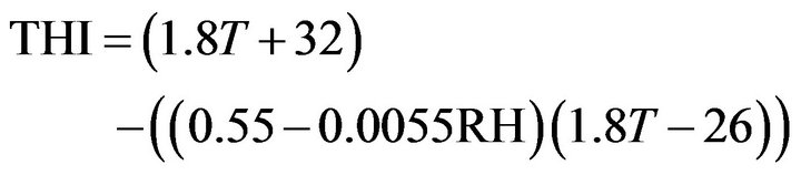
Temperature and humidity are the most important weather variables. To incorporate the effect of these weather variables together, a composite weather variable, temperature-humidity index, is defined as [19],
 (1)
(1)
whereTHI = Temperature-humidity indexT = Temperature (Degree Celsius) and RH = Relative Humidity (%).
The methodology requires the following steps for the identification of the weather sensitive component of electrical load.
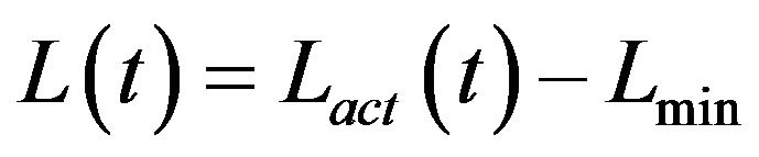
Step-1: In the first step, electrical load signal is decomposed using EMD technique. Before decomposition, the minimum value of the load is subtracted from the original load signal which results in modified load signal. It can be expressed as,
 (2)
(2)
whereL(t) = Modified load signal or variable load signal.
Lact(t) = Actual load signal.
Lmin = Minimum load during the considered period.
This subtraction operation is performed because the weather sensitive portion of the electrical load is hidden inside the envelope of the original load signal. To apply EMD on L(t) its upper envelope and lower envelopes are identified. The mean of the upper and the lower envelopes is determined and this mean is subtracted from the modified load signal. This is the first iteration to get first IMF. The iteration process continues until the first IMF is separated from the modified load signal. Further, this decomposition process continues. After decomposing L(t) using EMD technique, a finite number of IMFs and a residue, Re(t) are produced. Note that, Re(t) contains all positive values and the IMFs contain both positive and negative values.
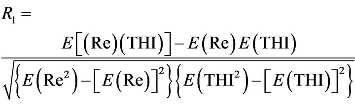
Step-2: Since electrical load signal can not be negative in magnitude, so at the second step, the correlation coefficient between the residue signal and the weather variable THI(t) is determined. In what follows Re(t) and THI(t) will be represented by Re and THI, respectively for clarity. The correlation coefficient of Re and THI is expressed as,
 (3)
(3)
where R1 = Correlation coefficient of Re and THI.
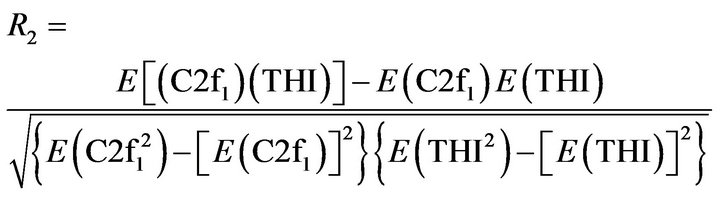
Step-3: In the third step, Re and last decomposed component of load, IMFn are combined to generate a new load signal, C2f1. That is,
 (4)
(4)
Then the correlation coefficient between C2f1 and THI is determined. Mathematically it is expressed as,
 (5)
(5)
whereR2 = Correlation coefficient of C2f1 and THI.
Step-4: In this step, Re and IMFn − 1 are combined to generate a new load signal, C2f2. That is,
 (6)
(6)
Then the correlation between C2f2 and THI is determined. Mathematically it is expressed as,
 (7)
(7)
whereR3 = Correlation coefficient of C2f2 and THI.
Step-5: Following the similar vein, residue signal is added to all the possible combinations of the IMFs and the corresponding correlation coefficient between each combination and THI is determined.
Step-6: In this step, the maximum value among the correlation coefficients  is determined. That is,
 (8)
(8)
Step-7: In this step, the value of the signal that corresponds to the maximum correlation coefficient is evaluated. This signal represents the weather sensitive portion of the electrical load.
3. Numerical Example
A numerical example will amply clarify the proposed methodology. For example, the daily peak load of Dhaka zone of Bangladesh Power System (BPS) of the year 2012 is considered here. The weather sensitive portion of these peak values will be evaluated by applying the proposed methodology. For better assimilation, every step of the proposed methodology is discussed chronologically.
a) The daily peak load and average THI of the year 2012 is presented graphically in Figure 1. THI is multiplied by 15 in order to plot peak load (PL) and THI on the same graph.
The correlation between daily peak load and average THI is 0.50% or 50%. So it is certain that a portion of the daily peak load is generated due to weather variables like
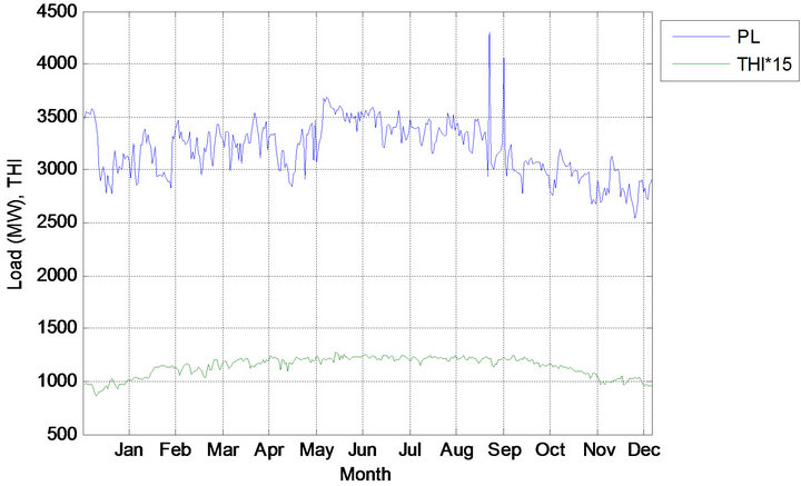
Figure 1. Daily peak load and average THI of the year 2012.
temperature and humidity. Now this weather sensitive portion of the load will be identified using the proposed methodology.
b) Minimum value over the whole year is subtracted from the daily peak values. It represented as, Daily variable load = Daily peak load – min (Daily peak load). The daily variable of the year 2012 is represented graphically in Figure 2.
c) Decomposition of the daily variable load of the year 2012 using empirical mode decomposition (EMD) technique results seven IMFs and a residue. The residue and the IMFs are presented graphically in the Figures 3-10.
d) Combining the seven IMFs, residue and the minimum value of the daily peak load, Figure 11 is obtained which actually represents the daily peak load of the year 2012. So, it is evident that, total variable load can be segregated into seven IMFs and a residue component.
e) Now, the correlation coefficient between the residue and combination of the residue and different IMFs of the variable load of the year 2012 is calculated. The values of these correlation coefficients are listed in Table 1.
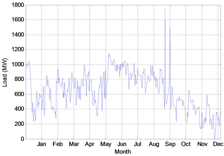
Figure 2. Daily variable load of the year 2012.
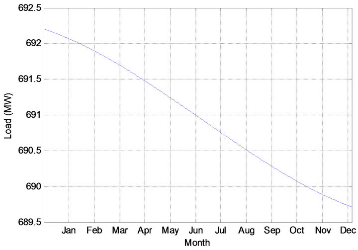
Figure 3. Residue of the variable load of the year 2012.
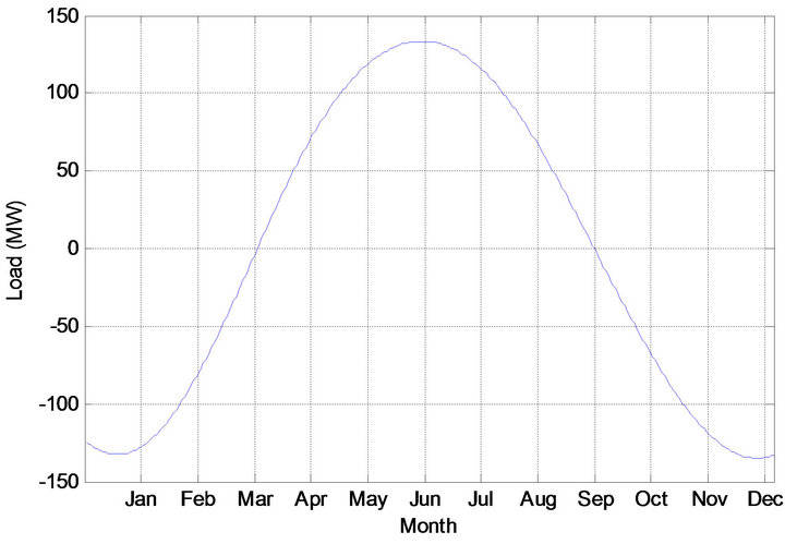
Figure 4. 7th IMF of the variable load of the year 2012.
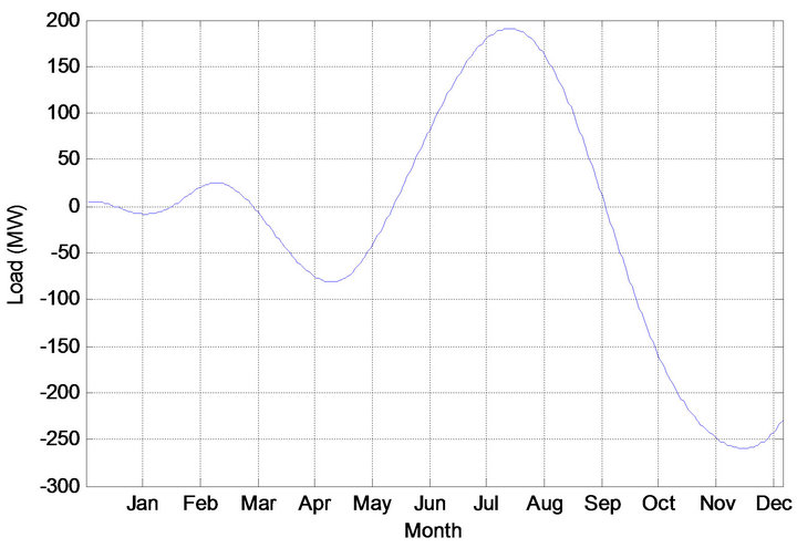
Figure 5. 6th IMF of the variable load of the year 2012.
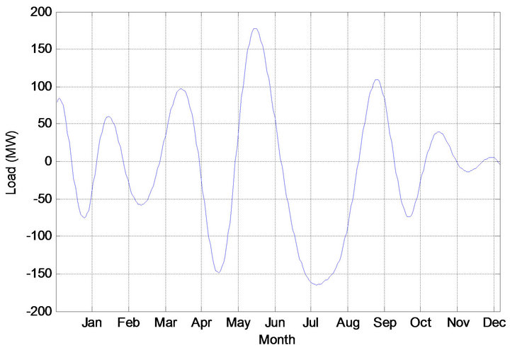
Figure 6. 5th IMF of the variable load of the year 2012.
f) Maximum value of the correlation coefficient is determined as: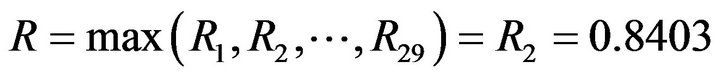 . The load signal corresponds to this maximum value is C2f1. So, the weather sensitive component of the daily peak load of the year 2012 is given by, Lw = C2f1.
The graphical representation of the weather sensitive portion of the daily peak load and average THI of Dhaka zone of BPS of the year 2012 is shown in Figure 12. THI
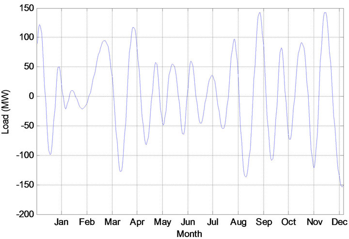
Figure 7. 4th IMF of the variable load of the year 2012.
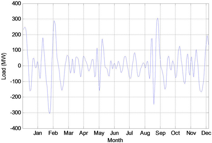
Figure 8. 3rd IMF of the variable load of the year 2012.
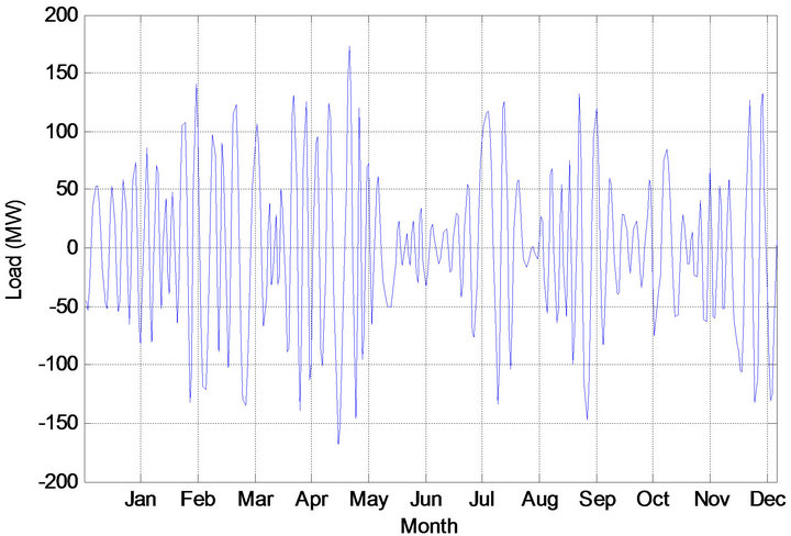
Figure 9. 2nd IMF of the variable load of the year 2012.
is multiplied by 5 to represent Lw and THI on the same graph.
4. Verification of the Proposed Methodology
The proposed methodology is applied to the historical daily peak load of Dhaka zone of BPS. For the verification of the proposed methodology, correlation coefficients (R) of Lw and THI of different months are measured
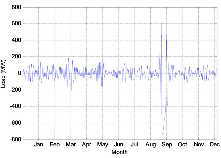
Figure 10. 1st IMF of the variable load of the year 2012.
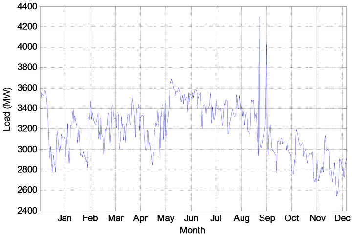
Figure 11. Combination of IMFs, residue and minimum value of the daily peak load of the year 2012.
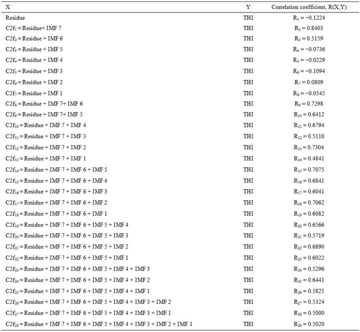
Table 1. Correlation coefficient.
for proposed methodology and weather-load model technique [9]. The result of the year 2012 and 2011 are shown in Figures 13 and 14, respectively.
The comparisons from Figures 13 and 14 clearly show
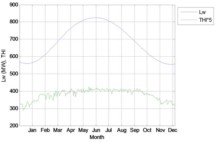
Figure 12. Weather sensitive portion of the daily peak load and average THI of the year 2012.
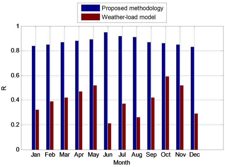
Figure 13. Comparison of correlation coefficients of the year 2012.
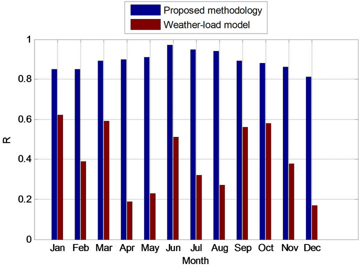
Figure 14. Comparison of correlation coefficients of the year 2011.
that the correlation coefficients between the weather sensitive portions of the load and THI for the proposed methodology are greater than that of weather-load model. It reveals that the weather sensitive portion of the load results from the proposed methodology is more accurate than that of weather-load model.
5. Results and Discussion
The salient features of the results those obtained by applying the proposed methodology are explained below for the year 2012. For close observation, average peak load, average THI and average weather sensitive component of the peak load of the year 2012 are presented graphically in Figures 15. Average peak load is divided by 2 and Average THI is multiplied by 5 in order to plot all the quantities on the same graph.
It is observed from Figure 15 that the average THI of February 2012 is much greater than that of January, 2012 but the average peak load of January, 2012 is not that much greater than that of February, 2012. The weather sensitive portion of February, 2012 is greater than that of January 2012 but their difference is very nominal (584.66 − 562.08 = 22.58 MW). In March, 2012 both average THI and average peak load are greater than that of February, 2012. As a consequence, the weather dependent portion of the load of the March, 2012 is greater than that of February, 2012. The same affiliation exists for the month of April, 2012 and March, 2012. This increasing drift of weather sensitive portion of the load continues up to June, 2012. From July, 2012 both monthly average peak load and monthly average THI starts decreasing. As a consequence, monthly average weather dependent portion of the load starts decreasing from July, 2012 and continues up to December, 2012.
The average Lw of January, 2012 and December, 2012 are very close. The average peak load of January, 2012 is grater than that of December, 2012 by 332 MW (3158.37

Figure 15. Average PL, average THI and average Lw of the year 2012.
MW - 2826.37 MW). But average THI of December, 2012 is greater than that of January, 2012 by 2.74 (66.68 - 63.94). As a consequence, the average weather sensitive portions of the load for these two months are very close to each other.
So it is clear that, the weather sensitive portion of the daily peak load varies with two parameters. One parameter is weather condition and the other parameter is daily peak load. If both parameters increase, the weather sensitive portion of the load increases. If both parameter decrease, the weather sensitive portion of the load decreases. If one parameter increases and other decreases, the weather sensitive portion of the load changes depending on the effect of dominating parameter.
To identify the weather non-sensitive portion of the load (NWL) of Dhaka zone of BPS, weather sensitive portion of the load is subtracted from the daily peak load. Monthly average NWL for the year 2012 is presented graphically in Figures 16. For close observation, corresponding average THI and average Lw are also plotted together. THI is multiplied by 5 and NWL is divided by 2 to facilitate all the quantities on same graph.
From the above graph, it is clearly observed that, the weather sensitive portion of the loads change sharply with THI. But the NWLs do not change with the weather conditions. For example, average THI of January and February, 2012 is 63.94 and 72.50, respectively. Average Lw of the peak loads of these two months are 562.08 MW and 584.66 MW, respectively. But the average NWL of these two months are 2596.29 MW and 2506.70 MW, respectively. That is, though average THI increases in February, 2012 than January, 2012 but average NWL decreases.
So it can be concluded that NWL are not affected by weather variables like temperature and humidity. It changes due to other factors such as population, education, industrial development, special events etc.
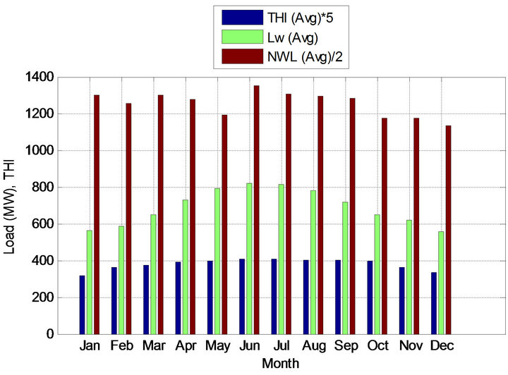
Figure 16. Average THI, average Lw and average NWL of the year 2012.
6. Conclusion
In this paper, a new methodology is proposed to identify the weather sensitive portion of the electrical load based on EMD technique. The developed methodology is applied to identify the weather sensitive component of the daily peak of Dhaka zone of BPS of the year 2012. The accuracy of the results is also measured by calculating correlation coefficient between THI and Lw for proposed methodology and weather-load model technique. In proposed methodology, the variable portion of the daily peak demand is decomposed into several components and these components have been correlated with weather parameters. As a result, the monthly variations of demand and weather conditions have been reflected properly. Finally it is observed that the weather sensitive portion of the electrical load varies with two parameters. One parameter is weather variables like temperature and humidity and the other parameter is total demand. Though the weather conditions are not that much different from a year to another, but it is observed that the weather sensitive portion of the load changes every year by a significant amount. This is because of the use of electrical appliances that generally increases year by year to mitigate the effect of the weather parameters.
REFERENCES
- R. L. Sullivan, “Power System Planning,” Mcgraw-Hill Book Company, New York, 1977.
- H. Chen, C. A. Canizares and A. Singh, “ANN-Based ShortTerm Load Forecasting in Electricity Markets,” Proceedings of the IEEE Power Engineering Society Transmission and Distribution Conference, Vol. 2, pp. 2011, 411- 415.
- S. Ruzic, A. Vuckovic and N. Nikolic, “Weather Sensitive Method for Short Term Load Forecasting in Electric Power Utility of Serbia,” IEEE Transactions on Power Systems, Vol. 18, No. 4, 2003, pp. 1581-1586. doi:10.1109/TPWRS.2003.811172
- J. W. Taylor and R. Buizza, “Neural Network Load Forecasting with Weather Ensemble Predictions,” IEEE Transactions on Power Systems, Vol. 17, No. 3, 2002, pp. 626- 632. doi:10.1109/TPWRS.2002.800906
- A. Khotanzad, M. H. Davis, A. Abaye and D. J. Maratukulam, “An Artificial Neural Network Hourly Temperature Forecaster with Applications in Load Forecasting,” IEEE Transactions on Power Systems, Vol. 11, No. 2, 1996, pp. 870-876. doi:10.1109/59.496168
- S. M. Moghaddas-Tafreshi and M. Farhadi, “A Linear Regression-Based Study for Temperature Sensitivity Analysis of Iran Electrical Load,” Proceedings of the IEEE International Conference on Industrial Technology, Chengdu, 21-24 April 2008, pp. 1-7. doi:10.1109/SUPERGEN.2009.5347944
- G. Y. Chen and J. T. Shi, “Study on the Methodology of Short-Term Load Forecasting Considering the Accumulation Effect of Temperature,” Proceedings of the International Conference on Sustainable Power Generation and Supply, Nanjing, 6-7 April 2009, pp. 1-4.
- E. Contaxi, C. Delkis, S. Kavatza and C Vournas, “The Effect of Humidity in a Weather-Sensitive Peak Load Forecasting Model,” Proceedings of the IEEE Power Systems Conference and Exposition, Atlanta, 29 October-1 November 2006, pp. 1528-1534.
- E. G. Contaxi and S. Kavatza, “Application of a Weather- Sensitive Peak Load Forecasting Model to the Hellenic System,” Proceedings of the IEEE Mediterranean, Vol. 3, 2004, pp. 819- 822.
- N. E. Huang, Z. Shen, S. R. Long, M. C. Wu, H. Shih, Q. Zheng, N. C. Yen, C. C. Tung and H. H. Liu, “The Empirical Mode Decomposition and the Hilbert Spectrum for Nonlinear and Non-Stationary Time Series Analysis,” Proceedings of the Royal Society A: Mathematical, Physical and Engineering Sciences, Vol. 454, No. 1971, 1998, pp. 903-995.
- K. I. Molla, K. Hirose and N. Minematsu, “Robust Determination of Periodic Correlation of Speech Signals Using Empirical Mode Decomposition and Higher-Order Spectra,” Proceedings of the Asia-Pacific Conference on Communications, Tokyo, 14-16 October 2008, pp. 1-5.
- K. Khaldi, M. T.-H. Alouane and A.-O. Boudraa, “Speech Denoising by Adaptive Weighted Average Filtering in the EMD Framework,” Proceedings of the International Conference on Signals, Circuits and Systems, pp 1-5.
- N. Chatlani and J. J. Soraghan, “Speech Enhancement using Adaptive Empirical Mode Decomposition,” Proceedings of the IEEE International Conference on Digital Signal Processing, Monastir, 7-9 November 2008, pp. 1- 6.
- M. Kiamini, S. Alirezaee, B. Perseh and M. Ahmadi, “Elimination of Ocular Artifacts from EEG Signals Using the Wavelet Transform and Empirical Mode Decomposition,” Proceedings of the International Conference on Electrical Engineering/Electronics, Computer, Telecommunications and Information, Pattaya, 6-9 May 2009, pp. 1094- 1097.
- Z. D. Zhao and C. Ma, “A Novel Cancellation Method of Power Line Interference in ECG Signal Based on EMD and Adaptive Filter,” Proceedings of the IEEE International Conference on Communication Technology, Hangzhou, 10-12 November 2008, pp. 517-520.
- X. J. Guo, X. P. Wu and D. X. Zhang, “Motor Imagery EEG Detection by Empirical Mode Decomposition,” Proceedings of the IEEE International Joint Conference on Computational Intelligence and Neural Networks, Hong Kong, 1-8 June 2008, pp. 2619-2622.
- P. F. Diez, V. Mut, E. Laciar, A. Torres and E. Avila, “Application of the Empirical Mode Decomposition to the Extraction of Features from EEG Signals for Mental Task Classification,” Proceedings of the IEEE International Conference on Engineering in Medicine and Biology Society, Vol. 2009, 2009, pp. 2579-2582.
- T. Q. Zhu, L. Y. Huang and X. Z. Tian, “Epileptic Seizure Prediction by Using Empirical Mode Decomposition and Complexity Analysis of Single-Channel Scalp Electroencephalogram,” Proceedings of the IEEE International Conference on Biomedical Engineering and Informatics, Tianjin, 17-19 October 2009, pp. 1-4.
- http://www.dairynz.co.nz