Communications and Network
Vol.2 No.1(2010), Article ID:1276,10 pages DOI:10.4236/cn.2010.21001
Using the Power Control and Cooperative Communication for Energy Saving in Mobile Ad Hoc Networks
1College of Information Science and Technology, Donghua University, Shanghai, China
2Department of Computer Science and Software Engineering, Monmouth University, West Long Branch, NJ, USA
E-mail: chunjiechen@mail.dhu.edu.cn, dazhilou@163.com, deminli@dhu.edu.cn, jwang@monmouth.edu
Received October 10, 2009; accepted November 11, 2009
Keywords: minimum spanning tree, traffic capacity, energy savings, cooperative communication
ABSTRACT
In this paper, we investigate the energy saving problem in mobile ad hoc network, and give out an improved variable-range transmission power control algorithm based on minimum spanning tree algorithm (MST). Using previous work by Gomez and Campbell [1], we show that in consider of node’s mobility, the previous variable-range transmission power control based on minimum spanning tree algorithm can not support nodes’ mobility in mobile ad hoc network. For this reason, we give out an improved variable-range transmission power control algorithm to support node’s mobility and solve asymmetric graph problem. To save more energy without changing the topology of the network, we give out two new data transmission me-chanisms based on the idea of cooperative communication. The results of this paper enhance the possibility of using variable-range transmission power control in mobile ad hoc networks.
1. Introduction
Energy saving problem is a very important issue in wireless ad hoc networks, because the transmission power impacts not only the connectivity but also the traffic capacity of the network. Choosing a higher transmission power can increase the connectivity and performance of the network, but reduce traffic capacity on the physical layer and energy on the network layer. Obviously, it’s a trade-off problem. Today, the design of protocols for wireless ad hoc networks is primarily based on common-range transmission control, such as the work by Santi et al. [2,3]. But systems based on common-range transmission control [3] usually assume nodes are homogeneously distributed. For some nodes, the topology will be too sparse with the risk of having network partitions. For other nodes, the topology will be too dense, resulting in many nodes competing for transmission in a shared medium. This problem is discussed in [4], where the authors propose a method to control the transmission power levels in order to control the network topology. In [1], Gomez and Campbell show how variable-range transmission control can improve the overall network performance and suggests the design of MAC and routing protocols for wireless ad hoc networks should base on variable-range power control, not on common-range transmission control which is prevalent today. But in consider of node’s mobility, using previous variablerange power control still have some problems such as the traffic capacity tends to be zero because the area of overlapping region is zero. Furthermore, because in variable-range control, all nodes use different transmission powers, this also may lead to asymmetric graph problem.
In this paper we give out an improved power control algorithm based on minimum spanning tree to solve these problems and provide the possibility of using variable-range transmission power control in wireless ad hoc networks.
Furthermore, we investigate the effect of cooperative communication mechanism on energy saving for ad hoc networks. Many recent cooperative communication mechanisms change node’s transmission power such as in [5] to save energy. But as Cardei said, using cooperative communication to control transmission power is an NPComplete problem. Then we give out two new data transmission mechanisms based on the idea of cooperative communication. We prove these two mechanisms can solve the energy saving problem by reducing the transmission time rather than changing node’s transmission power so it can be realized easily.
The structure of this paper is as follows. In Section 2 we give out an improved variable-range transmission power control algorithm to support node’s mobility and solve asymmetric graph problem. Given the topology of the network, in Section 3 we will describe two new data transmission mechanisms Sequence Data Check Transmission mechanism (SDCT) and Nearest Data Check Transmission mechanism (NDCT) based on our cooperative communication mechanism in detail to save more energy without changing the topology. To show the advantage on energy saving of our new data transmission mechanisms along with numerical simulation, in Section 4, we give out their mathematical model and some basic suppose. Through these mathematical models, we compute the average hop of traditional data transmission mechanism (TDT), SDCT and NDCT. Finally, we present some concluding remarks in Section 6.
2. Improved Variable-Range Power Control Algorithm
According to Gomez and Campbell [1], we find whether the algorithm can support node’s mobility, depending on how large the area of overlapping region is. So can we enlarge the transmission power value in variable range control to a certain value? How to choose the bound of this value? How to deal with the asymmetric graph problem?
2.1 Traffic Capacity Using Previous Variable-Range Transmission Control in Mobile Network
In a mobile ad hoc network, nodes always move in a fast speed, this produces extra signaling overhead which consume a large part of network resources. In [1], Javier give out an equation to compute the signaling overhead of route maintenance. Javier suggested using previous variable-range transmission control based on minimum spanning tree lead to the time of a node remains in overlapping region b tends to zero. Figure 1 highlights one of overlapping regions.
It is obvious, because the network is built by minimum spanning tree, so1-hop nodes are always on the edge of their source nodes’ coverage range and the area of the overlapping region b is zero. We prove this point by (15).
 (1)
(1)
Because the average number of route-repair events persecond per route, proportional to ,
,  is very large and because the traffic capacity of variable-range control
  tend to be a const when
 , so the capacity available to nodes for data transmission
  is very small. This means the topology of the network is always changing and the whole wireless channel is occupied by
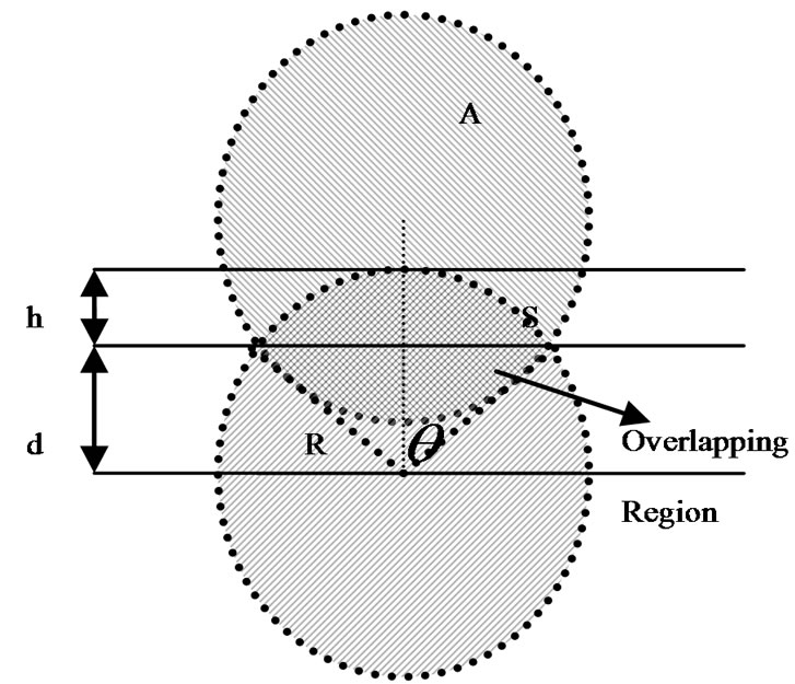
Figure 1. Overlapping region between two nodes
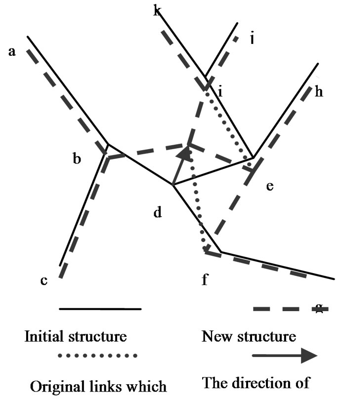
Figure 2. Topology change when node moves
the signaling overhead caused by route maintenance.
2.2 Improved Minimum Spanning Tree Algorithm for Upper Bound
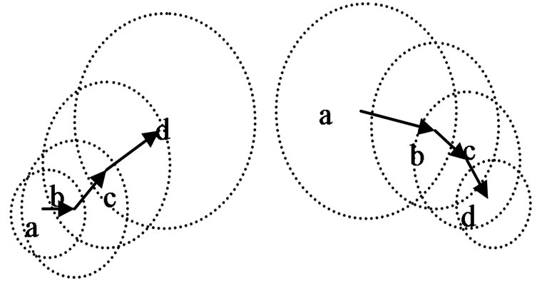
We can see the key problem of previous variable-range transmission control is caused by route maintenance, so we must first discuss in which conditions the route of the network will be updated. Figure 2 shows that the change of topology in an ad hoc network whose nodes are distributed randomly. When node d moves in that direction shown by the arrow, the network will form a new minimum spanning tree shown by doted lines.
The original links of  and
and  are now disconnected and the new links of
  and
and  are established. By Figure 2, we find route maintenance occur in two conditions:
1) Forwarding nodes move out the region which is covered by transmitter node at the upper bound of transmission power.
2) Current structure of the network is no longer a minimum spanning tree and need to rebuild a new minimum spanning tree.
We can see the problem is to choose a suitable upper bound for node’s transmission power.
By analyzing, we find when a node moves, the length of edges which connected to this node will change, and when this length beyond the shortest edge of its 1-hop nodes, which results in the nodes are not connected in original minimum spanning tree, the network needs to rebuild and the route needs to be updated.
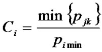
Highlight from this point, we get the conclusion that the upper bound for a node’s transmission power should be set to the value of the shortest edge of its 1-hop nodes which are not connected in original minimum spanning tree. But, there is an extreme condition that the upper bound may be much larger than original transmission power. To keep the superiority of minimum spanning tree algorithm, there must be a threshold to limit the upper bound. If we use  to denote the minimum transmission power of node i in minimum spanning tree, to every node i,
 (2)
(2)
where j is 1-hop node of node i and k is 1-hop node of node j,  is the transmission power between node j and node k. Because
 is the minimum transmission power of node i in minimum spanning tree. We set
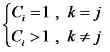
and there are two cases:
 (3)
(3)
where  means node j has only one 1-hop node, and this 1-hop node is node i.
Then we get the threshold
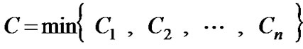 (4)
(4)
Finally we set the upper bound of the node’s transmission power to:
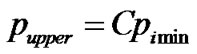 (5)
(5)
where  stands for the upper bound of transmission power according to the improved algorithm.
2.3 Adaptive Transmission Power Control for Lower Bound
To support node’s mobility, we know node’s transmission power should larger than that got by minimum spanning tree. But the upper bound  may be much larger than
 , considering that the mobility of mobile nodes is limited by physical restrictions, it is not necessary to enlarge the transmission power to
  in just one step. It can be a gradually increment process.
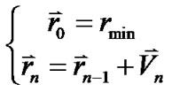
Considering that a mobile node’s future location and velocity are likely to be correlated with its past and current location and velocity, according to Ben Liang and Zygmunt J. Haas [6], we use a 2-D Gauss-Markov mobility model to estimate node’s future distance from its back-warding node.
In this 2-D Gauss-Markov mobility model, the velocity of a mobile is represented by the random vector:
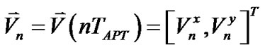 (6)
(6)
where  is the time interval used to sense and compute. Define memory level :
 (7)
(7)
where  are parameters correlated to
 .
.
Then, the 2-D velocity process can be expressed as follows:
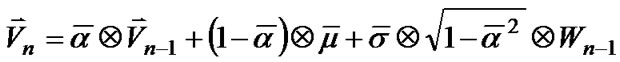 (8)
(8)
where  denotes element-by-element multiplication,
 and
and is the variance of
 ,
,
 is its mean.
  is an uncorrelated Gaussian process with zero mean and unit variance and is independent of
 .
.
For simplicity of presentation, one may further assume that the velocity has the same memory level, the same asymptotic mean, and the same asymptotic standard deviation in both dimensions. In this isotropic case (8) becomes:
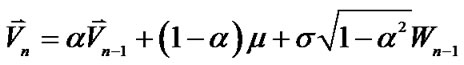 (9)
(9)
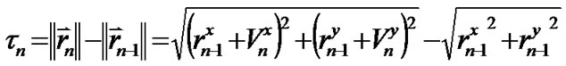
If we use 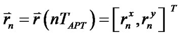 to denote the distance from back-warding node to its 1-hop node, we get:
 (10)
(10)
Then we choose the increment of transmission range, denoted by  shown in Figure 3, as the step of adaptive mechanism:
 (11)
(11)
So within a slot of , 1-hop node is still in the transmission range of transmitter node to ensure network connectivity until the transmission range achieve the upper bound. When a node’s transmission power approximates to its upper bound, it can broadcast to the whole network to ready for rebuild the minimum spanning tree. So the adaptive and heuristic algorithm can meet the networks switch for route and the requirement for QoS.
Now compare the transmission energy and traffic capacity between common-range control, previous variable-range control and improved variable-range control.
2.3.1 Transmission Energy
We know in common-range control, the transmission power, denoted by  must meet the restriction:
 (12)
(12)
to make sure that every node is connected to the network.
Here we use to stand for the transmission power of improved variable-range control. By using adaptive mechanism, we get
 (13)
(13)
where  is the extra transmission power of node i that needed to enlarge the transmission range of minimum spanning tree with one step.
The total transmission energy of one route in previous variable range control is
 (14)
(14)
We can use (12) and (13) to compute the total transmission energy of one route in the network. We get the total transmission energy of common-range control
 (15)
(15)
and the total transmission energy of improved variablerange control
 (16)
(16)
From (12), (13), (14), (15) and (16), compare the transmission energy between common-range control, previous variable-range control and improved variablerange control, we get Theorem 2.1 The total transmission energy of improved variable-range control is between common-range control and previous variable-range control:

 .
.

 (17)
(17)
2.3.2 Traffic Capacity of Improved Minimum Spanning Tree Algorithm
We can see, after enlarge the transmission power of minimum spanning tree to the upper bound of , the parameter h is increased from 0 to
 , using (6) we deduce the signaling overhead of the improved variable-range control.
From (3) and (4) we know C is a constant larger than 1, so  is a constant too. Compare to the signaling overhead of previous variable-range control which is tend to infinite, it’s much smaller.
From (2), (4) and (12) we know
 (19)
(19)
and  decreases as the parameter h increases.
According to the analysis and comparison above, we know the improved variable-range control can balance the transmission energy and signaling overhead in mobile ad hoc networks and it is an optimization of energy-saving and traffic capacity, it improves the mobility of the network greatly at the cost of a little more transmission power.
2.4 Asymmetric Graph
Different from common-range control, in variable-range control, all nodes use different transmission power, this may lead to the final structure of the network is an asymmetric graph, like Figure 3. To solve this problem, we select the sequence of transmission ranges from source node to the destination node to be an incremental sequence Here we use the method of “Incremental” which means if the transmission range of forwarding node is smaller than the source node, we use the transmission range of the source node to replace the transmission range of forwarding node. By this way, we ensure the sequence of transmission ranges from node to the destination node is monotone-up and the structure of the network in Figure 4 changes to Figure 5 by the monotone-up selecting method.
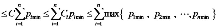
There are two extreme situations shown in Figure 6a and Figure 6b. In Figure 6a, the sequence of transmission ranges from source node to the destination node is monotone-up and In Figure 6b the sequence of transmission ranges from source node to the destination node is monotone-down. After “Incremental”, we get the new transmission ranges shown by Figure 6c and Figure 6d. Then we get that:
Theorem 2.2 The total transmission power of the network after “Incremental” is between improved variablerange control and common-range control.
 (18)
(18)
Proof: If we use  to stand for the sequence of transmission ranges from source node to the destination node after adaptive power control, then the sequence of transmission ranges from source node to the destination node after coverage is
 In the condition of
  we get the transmission power of forwarding node is

Figure 3. Increment step of transmission range

Figure 4. Asymmetric structure of the network
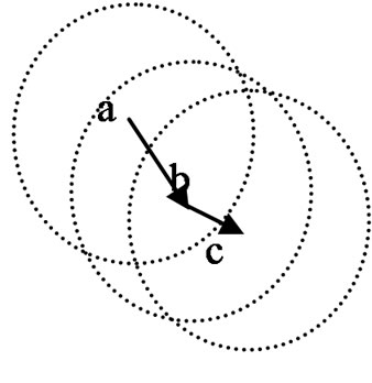
Figure 5. Monotone-up transmission range
 (20)
(20)
And on the other hand, when the condition is 
 the transmission power for next hop will be
 (21)
(21)
And (21) stand for once change on the sequence of transmission ranges from source node to the destination node after adaptive power control. Because this change occurs when , so the total transmission power will increase after this change.
If original sequence is monotone-up, the number of change is zero which is the smallest. On the other hand, if original sequence is monotone-down, the number of chan
 (a) (b)
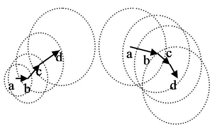 (c) (d)
Figure 6. (a) Condition of monotone-up; (b) Condition of monotone-down; (c) Evolution from Figure 6a after “Incremental”; (d) Evolution from Figure 6b after “Incremental”
ge is  which is the largest. And if the original sequence is monotone-down, the final sequence of transmission power is
where
 (22)
(22)
From (12) we can see  is smaller than
When the original sequence is neither monotone-up nor monotone-down, the number of change is between zero and , so the total transmission power after “Incremental”, denoted by
  is:
is:
 (23)
(23)
Thus, by enlarging the transmission range to the upper bound , adaptive transmission rang and the “Incremental” of transmission range, we have solved the traffic capacity tends and asymmetric graph problem of previous variable-range control mentioned above.
3. Cooperative Communication for Energy Saving
We all know that energy is the product of transmission power and transmission time, so the transmission energy is related to not only the transmission power but also the transmission time which is decided by the length of data. We usually choose changing transmission power to optimize the network, but changing transmission power also lead to the change of network topology. In [5], Cardei proves it’s a NP-complete problem. So after get the topology of the network by improved variable-range control, the transmission power can not be changed further, one way to save more transmission power is to control the time of transmission. Here we use the cooperative communication mechanism because it can save transmission power without changing the topology of the networks (related to transmit time or length of data).
3.1 Cooperative Communication Mechanism
In [7], Agarwal introduced two parameters related with SNR: , which is the threshold needed to successfully decode the packet payload, and
 , which is the threshold required for a successful time acquisition. In [5] Cardei assumes a packet received with a SNR
 , is: 1) fully received, if
 ; 2) partially received if
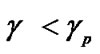 , and 3) unsuccessfully received, if
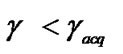 . And in Cardei’s cooperative communication model, consider the packet is fully received when
 (24)
(24)
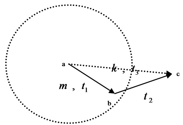
Figure 7. Node c receive k packets in m packets from node a
where  is the transmission power of node k,
  is the distance between node k and node j, and
  is a communication medium dependent parameter. But if there are overlapping parts of partial data, can (24) stand for full reception of the packet?
Based on this question, we give out our own cooperative communication mechanism.
We consider that messages are divided into several packets. If forwarding nodes are in the area of source node’s transmission range, all packets can be transmitted to the 1-hop node of source node completely and correctly. But when forwarding nodes, such as 2-hop node and 3-hop node, are out of the transmission range of source node, only a part of packets can reach 2-hop node and 3-hop node, and among these partial data, some packets will fail because of distortion. We can see from Figure 7 if there are m packets to be transmitted from node a to node c, there will be k packets reach node c when node a transmits all these packets to node b. After validation, we can know which packets are correct. And when node b transmit data to node c, we do not need to retransmit these correct packets, and only transmit those packets which are not received or incorrect.
This mechanism can save more transmission energy without change the topology of network.
3.2 Mathematical Model
To simplify, we just consider the influence of source node on its 2-hop nodes.
Noting that wave transmits at the same speed in the same medium, from Figure 7, we know 
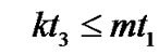 (25)
(25)
so
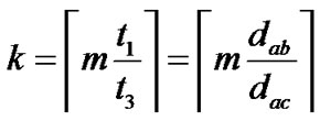 (26)
(26)
where  and
and  is the time need to transmit per packet from node a to node b and from node a to node c.
Though there will be k packets reach node c in Figure 7, because of noise, some packets will fail because of distortion and how many packets can reach node c correctly is depend on the symbol-error-rate (SER) which is relate to the signal-to-noise ratio (SNR).
In [8], Ahmed and Weifeng Su give out a model of the relationship between symbol-error-rate (SER) and signal-to-noise ratio (SNR):
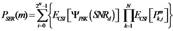 (27)
(27)
The model in [8], always choose the source node as the most reliable node, but in multi-hop network, the distance between source node and destination node is usually very long, this lead to the direct link between source node and destination node can not meet the requirement of high enough SNR, or there is even no direct link between source node and destination node. Another important point is that in this model, there are  possible network states, this means in most states, there are some nodes on the route are not in state and they do not relay the copy of data to other nodes. But as the nodes on the route form a chain, if there is one node do not relay the copy of data to its next node, the data can not reach the destination node correctly. So we should improve this model according to our improved routing strategy.
In our cooperative communication model, all packets can be transmitted to the 1-hop node of source node completely and correctly, so after the packets reached the 1-hop node, we can treat it as a new source node for the rest route. Compared to the source node, 1-hop node is closer to the destination node so the SNR of 1-hop is higher than the SNR of the source node. So there is only one network state in our cooperative communication model that all nodes are in state and relay the copy of data to other nodes.
So according to our model, we can simplify (27) to:
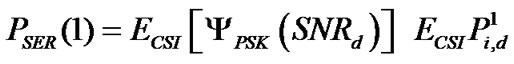 (28)
(28)
where i is 1-hop node of the source node and d is the destination node. When just consider the influence of source node on its 2-hop node, the destination node is also the 2-hop node of the source node.
We assume that whether a packet can be received corrected is independent on other packets, and use function  to denote whether the
  th packet is received correctly.
 (29)
(29)
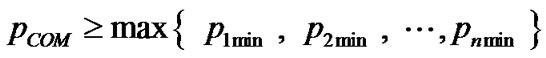
thus the number of packets  that can be received correctly is
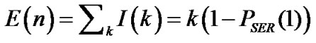 (30)
(30)
So for every hop in the route, we can save the transmission energy used to transmit  packets.
3.3 Two New Data Transmission Mechanisms Based on Cooperative Communication
After we prove the cooperative communication mechanism can save energy by shorting the time of transmission, we now give out two new data transmission mechanisms based on it.
3.3.1 Sequenced Data Check Transmission Mechanism
In this mechanism, the whole transmission process is sequenced according to the order of nodes from source to destination. The concrete process can be described as follow:
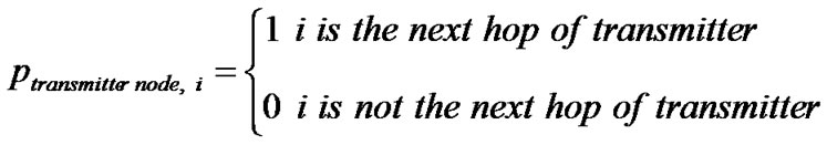
Step 1: The source node start the transmission process by sending route requiring signal (RRS) to the destination through forwarding nodes.
Step 2: Then the destination node return a route confirm signal (RCS).
Step 3: Source node will first send an inquire signal to its next hop to ask which packets does next hop need.
Step 4: After next hop return the packets ID which it has not received correctly, the source node begins to transmit these packets to next hop. Other nodes on the route receive these packets at the same time. They can know which packets are correct by checking.
Step 5: After all packets reach next hop return an ACK to the transmitter node and get ready to transmit data to its next hop.
Step 6: All forwarding nodes repeat Step 4–Step 5.
Step 7: If all packets reach the destination correct, the destination node will sent out a signal to acquire all nodes on the route to end this transmission process.
This mechanism is similar to recent point to point communication system, so it can be realized easily.
3.3.2 Nearest Data Check Transmission Mechanism
Though SDCT can save energy a lot, bet because the transmission process is ordered by nodes, the destination node can end the transmission process only after every node on the route received all data packets. Sometimes it is unnecessary and may lead to extra energy waste.
Thus we give out another data transmission mechanism:
Nearest Data Check Transmission (NDCT) to avoid this kind of energy waste. The main difference between SDCT and NDCT is: in NDCT, every node can send a route require signal to destination after it receive a correct packet and the destination node will choose the most reliable node (usually the nearest node) to relay. But in SDCT, for the  th relay, only the
  th node on the route can send a route require signal to destination after it receive all packets correctly. The concrete process is as follow:
Step 1: Source node start the transmission process by sending route requiring signal with first packet ID to the destination through forwarding nodes.
Step 2: When the destination node receives several route require signal, it will choose the nearest node to return a route confirm signal.
Step 3: Node which receives the confirm signal will send one packet to its next hop.
Step 4: After next hop receive this packet correctly, it will send out a route require signal to ask for transmitting this packet. This route requiring signal will keep until the destination node reply a clear signal to start the transmission process of next packet.
Step 5: All forwarding nodes repeat Step 2–Step 4.
Step 6: If this packet reach the destination node correctly, the destination node will send out a clear signal to acquire all nodes on the route to clear their route requiring signal and turn to the transmission process of next packet.
This mechanism can save more energy than SDCT but it is much more complex.
4. Mathematical Models of SDCT and NDCT
Given the whole process of data transmission, now we can use Markov process to build mathematical models for SDCT and NDCT.
Here we consider a route with K nodes. The route status at moment n is defined as
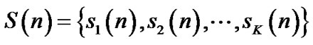 (31)
(31)
here  is the status of node i at moment n and
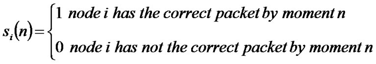
(32)
Obviously, and during the whole transmission process, there will be
  possible statuses from
  to
to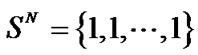 .
.
State transition probability matrix is:
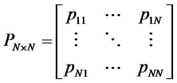 (33)
(33)
here is the probability the route status transmit from
  to
to .
.
According to the feature of Markov process, we know
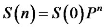 then
then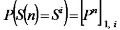 .
.
Here we first do some basic suppose: Suppose (1) The possibilities of every forwarding node receive a correct packet from transmitter node is independent of each other.
Then 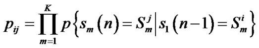 (34)
(34)
Suppose (2)
 (35)
(35)
where  is the probability of node I receive a correct packet from the transmitter node. Then
 (36)
(36)
 (37)
(37)
 (38)
(38)
thus  where
where  is the probability that the route status transmit from
  to
to  for the first time after n steps.
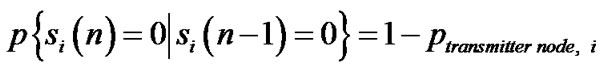
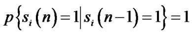
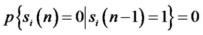
Suppose (3) The probability of every transmitter node transmit a correct packet to its next hop is 1:
 (39)
(39)
So we can easily conclude the status of route will reach  by most
  steps.
Given these three basic suppose now we can compute the average hops of traditional data transmission (TDT), SDCT and NDCT.
4.1 Traditional Data Transmission Mechanism
In traditional data transmission mechanism
(40)
and the transmission process will be ended at . Obviously
 (41)
(41)
Then the average hop of traditional data transmission mechanism is .
.
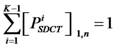
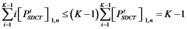
4.2 SDCT
In SDCT, the transmission process is sequenced by the order of nodes. So the transmitter can be denoted by
 (42)
(42)
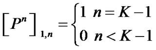
Because the destination node can end the transmission process until every node on the route received all data packets. So the transmission process will be ended at .
.
Then the average hop of SDCT is 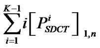
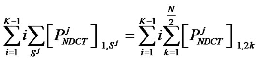
Theorem3.1 The average hop of SDCT is less than TDT Proof: Because
 (43)
(43)
so we get
 (44)
(44)
Theorem 1 is proved.
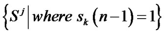
4.3 NDCT
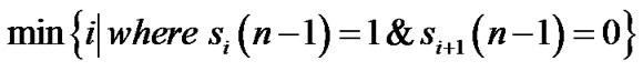
In NDCT, the destination node will choose the nearest node to which has the correct packet as the transmitter. So the transmitter can be denoted by
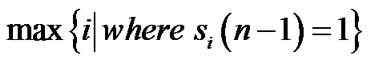 (45)
(45)
and the destination will end current packet transmission process as soon as the correct packet reach the destination node. So the transmission process will be ended at every status
 (46)
(46)
Then the average hop of NDCT is
 (47)
(47)
Theorem3.2 The average hop of NDCT is less than SDCT Proof: To compare the average hop of SDCT and NDCT, we should divide the transmission process into two cases:
1) The route status reaches  do not through
2) The route status reaches  through
In case 1), because both SDCT and NDCT end the transmission at , so their average hop are the same.
In case 2), according to suppose (2) 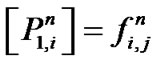
then we get

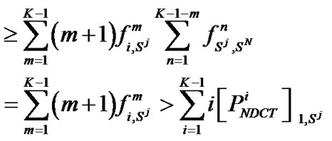 (48)
(48)
Theorem 2 is proved.
5. Numerical Simulation
To verify our theory, we do some simulation on the average hop of TDT,SDCT and NDCT.
Here we use a route of 4 nodes, and the state transition probability matrix is as follow:
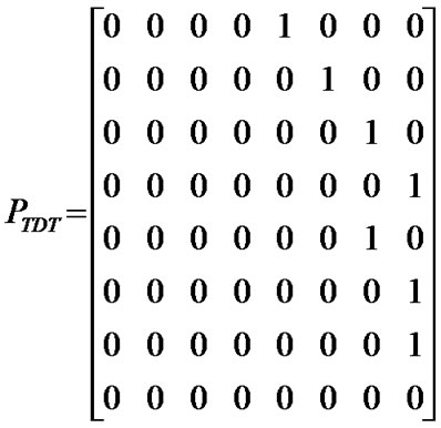

And

Table 1 shows the hops used to complete the transmission process of TDT, SDCT and NDCT and their probabilities.
Finally we get the average hop of TDT is 3, SDCT is 1.728 and NDCT is 1.648. Thus the advantage on energy saving of our new data transmission mechanism has been proved.

Table 1. Probabilities of hops used to complete the transmission process
6. Conclusions
In this paper, we give out some effective solutions to improve previous variable-range control such as improved minimum spanning tree algorithm, adaptive power control mechanism and the “Incremental” of transmission power. We prove the improved variable-range control is an optimization of traffic capacity and energy saving. The variable-range control method improves the performance of the mobile ad hoc networks efficiently at the cost of a little more transmission power. Furthermore we describe two new data transmission mechanisms based on our cooperative communication mechanism in detail and show their advantage on energy saving with numerical simulation. By these improvements, we provide the possibility of using variable-range transmission power control in wireless ad hoc networks.
7. Acknowledgements
This work is partially supported by Shanghai Key Basic Research Project under grant number 09JC1400700; NSFC granted number 70271001, China Postdoctoral Fund granted number 2002032191, Shanghai Fund of Science and Technology granted number 00JG05047, the Shanghai Key Scientific Research Project under grant number 05dz05036, and the fund of Engineering Research Center of Digitized Textile & Fashion Technology, Ministry of Education.
REFERENCES
- J. Gomez and T. Campbell, “Variable-range transmission power control in wireless ad hoc networks,” IEEE Transactions on Mobile Computing, Vol. 6, No. 1, pp. 87–99, 2007.
- P. Santi, D. M. Blough, and F. Vainstein, “A probabilistic analysius for the range assignmernt problem in ad hoc networks,” Proceeding ACM Mobihoc, pp. 212–220, August 2000.
- MANET, IETF Mobile Ad-Hoc Network Working Group, 2006, http://www.ietf.org/html.charters/manet-charter.html.
- R. Ramanathan and R. Rosales-Hain, “Topology control of multihop wireless network using transmit power adjustment,” Proceeding IEEE INFOCOM, pp. 404–413, 2000.
- M. Cardei, J. Wu, and S. Yang, “Topology control in ad hoc wirelsee networks using cooperative communication,” IEEE Transactions on Mobile Computing, Vol. 5, No. 6, 2006.
- B. Liang and Z. J. Haas, “Predictive distance-based mobility management for multidimensional PCS networks,” IEEE/ACM Transactioons on Networking, Vol. 11, No. 5, pp. 718–732, October 2003.
- M. Agarwal, J. H. Cho, and J. Wu, “Energy efficient broadcast in wireless ad hoc networks with hitch-hiking,” Proceeding IEEE INFOCOM, 2004.
- A. K. Sadek, W. F. Su, and K. J. R. Liu, “Multinode cooperative communications in wireless networks,” IEEE Transactions on Signal Processing, pp. 341–355, 2007.