Advances in Pure Mathematics
Vol. 3 No. 3 (2013) , Article ID: 30969 , 8 pages DOI:10.4236/apm.2013.33044
One Step Forward, Two Steps Back: Biconvergence of Washed Harmonic Series
Department of Mathematics, George Mason University, Fairfax, USA
MCSP Department, Roanoke College, Salem, USA
Email: cdavi3@gmu.edu, taylor@roanoke.edu
Copyright © 2013 Christopher M. Davis, David G. Taylor. This is an open access article distributed under the Creative Commons Attribution License, which permits unrestricted use, distribution, and reproduction in any medium, provided the original work is properly cited.
Received February 5, 2013; revised March 8, 2013; accepted April 6, 2013
Keywords: Harmonic Series; Biconvergence; Non-Integer Series
ABSTRACT
We examine variations of the harmonic series by grouping terms into “washings” that alternate sign with the number of terms in a washing growing exponentially with respect to a fixed base. The bases x = 1 and x = ∞ correspond to the alternating harmonic series and the usual harmonic series; we first consider other positive integral bases and further we consider positive real number bases with a unique way to make sense of adding a non-integral number of terms together. In both cases, we prove a remarkable result regarding the difference between the upper and lower convergent values of the series, and give some analysis of this behavior.
1. Introduction
Possibly the simplest and most beautiful infinite series to conceptualize, the harmonic series intertwines a world of raw mathematical fortitude with that of elegant musical theory. Holding its origins in ancient Greece, the harmonic series was first proven to diverge in the 14th Century by Parisian scholar Nicole Oresme [1,2]. In 1672 and 1689, respectively, Mengoli and Bernoulii provided additional unique proofs of the series’ divergence. With such a basic form, the harmonic series yields itself to various manipulations and interpretations. One of the more fascinating alterations to the harmonic series, presented by A. J. Kempner in 1914, included the idea of omitting terms with a nine in the denominator [3]. Although this may seem to be insignificant when speaking of an infinite sum, it actually produces a very interesting result— remarkably, the sum converges! More recently, number theorists and theoretical physicists have taken an interest in double, triple, and multiple harmonic series [4-7]. To build, for example, the double harmonic series, consider the positive integer lattice ; the series is then the sum of all terms of the form
  taken over this lattice. Here we present our own manipulation—an altered version of this classic series as well. We won’t be omitting terms, but simply altering the way in which the series is summed—the “walk” of the series, if you will.
Our paper will be organized in the following fashion. Section 2 will introduce our modified walk; the way in which we wish to view our altered harmonic series. Section 3 expands upon our work and progresses to the general positive integer case. The general case for all real numbers is then discussed in Section 4 followed by an analysis of our work in Section 5. Further questions are then posed in Section 6. Although pivotal in musical theory, the harmonic series, we believe, is a cornerstone upon which new mathematics is built.
2. A Washed Harmonic Series
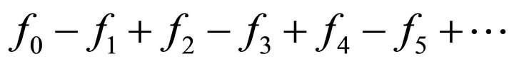
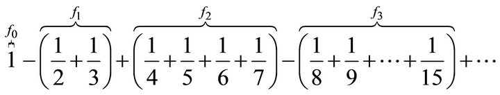
Let us consider the following series that involves the terms of the harmonic series, but with an interesting twist:

Upon first notice of this harmonic-type series there are a few observations. The terms of this series have had their signs (±) adjusted so that the first term is added, the next 2 terms are subtracted, the next 4 terms are added, the next 8 terms are subtracted, and the next 16 terms are added. This process continues for this infinite series where we either add or subtract terms in segments of powers of 2.
In terms of “walking through a room” one can think of themselves as standing on the opposite side of a room and starting to walk towards the other side (where the door might be). After going slightly more than 83%
 of the way to the other side, you decide to turn around and walk back towards your starting point. You travel a distance of almost 76% of the length of the room
 . You again reverse directions and continue this process.
We will call this particular series the washed harmonic series of base 2. There are obviously some natural questions to be asked. As one traverses the room is there any point at which walking would cease; that is to say, does this series converge? If so, then what point does this walking cease and/or series converge to? Or would the one walking leave the confines of the room; in other words, does the series have partial sums below 0 or above 1? Perhaps none of these things would happen and instead one would forever walk between two fixed spots, in essence would this “biconverge”?
To establish a notion of biconvergence, from any series which has both positive and negative terms we can construct an alternating series that we call the “washed” series associated with the original (“washed” after the up and down motion of washing clothes prior to our modern day washing machines).
Definition 2.1. To construct the washed series for a series
we define  to be the sum of all of the first positive terms (that is,
  where each
  and
and ),
),  to be the negated sum of all of the next negative terms (that is,
 where each
  and
and
 ),
),  to be the sum of all of the next positive terms,
  to be the negated sum of all of the next negative terms, and so on and so forth. The washed series associated to the original series is then
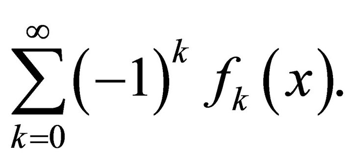
Definition 2.2. A (washed) alternating series given by
 is said to biconverge if

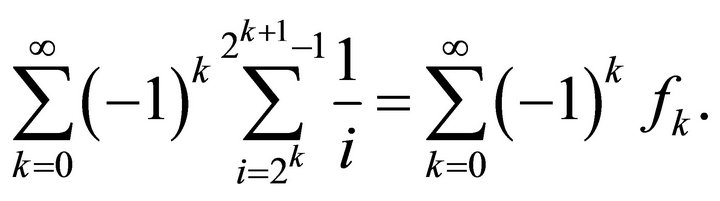
Observe that a biconvergent series, as  goes to infinity, will oscillate between an upper partial sum and a lower partial sum. The limit of the upper partial sum will be called the upper convergent value and the limit of the lower partial sum will be called the lower convergent value. To answer some of the questions regarding the washed harmonic series with base 2, it helps to formulate this series in a concise way. Define the mapping
 by
by 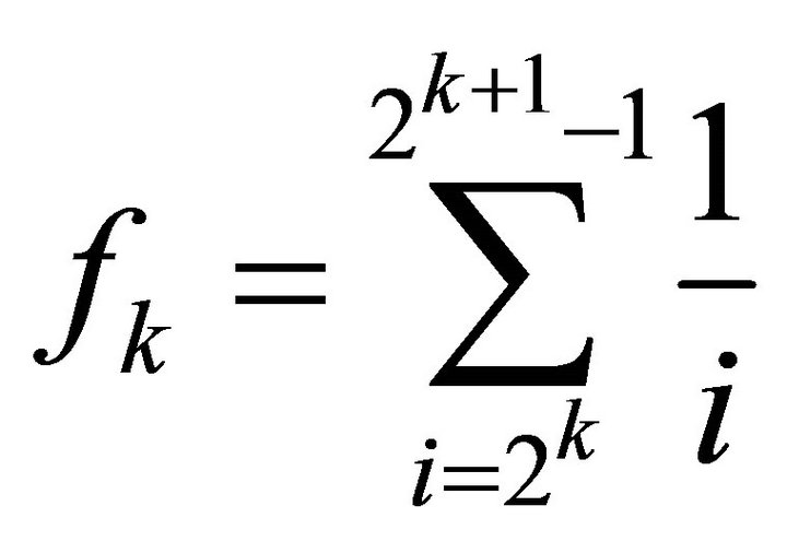 and notice that our series is
To note this explicitly, we see
can be expanded as
Proposition 2.1. We have

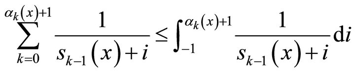
Proof: Since the function  is decreasing, we have the inequality
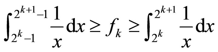
for all  (since we only care about long-term behavior, the term
  is irrelevant). Since
and
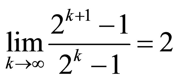
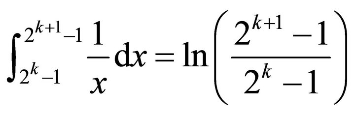
we have that
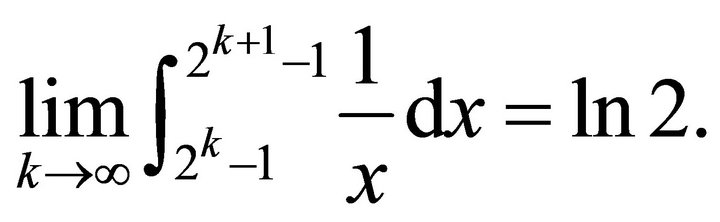
Apply the same argument to the integral on the righthand side of the inequality to see that
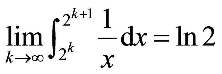
and apply the squeeze theorem to finish the proof.
This proposition shows that this series is indeed biconvergent; the person walking back and forth across the room will eventually be walking a distance of  (with respect the distance across the room being 1) in each step before changing directions. Perhaps the most natural question now is what are the two biconvergent values? That is, what is the upper convergent value, and what is the lower convergent value. To analyze this series further, let us introduce a definition.
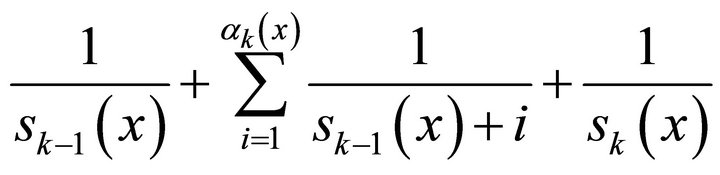
Definition 2.3. For a series defined as
the term  will be called a washing of the series, while the term
  will be called a complete washing of the series.
A list of values for the partial sum of the series after each washing can be found in Table 1. Observe the oscillating behavior in values as the number of washings increases.
3. The General Positive Integer Case
We now consider a more general case. In the above case, the washing sizes are powers of 2; consider what happens when the washing sizes are powers of an arbitrary integer . That is, we again start with the first term of the harmonic series, then subtract the next
 ![]() terms of the harmonic series, followed by adding the next
terms of the harmonic series, followed by adding the next  terms of the harmonic series, and so-on and so-forth.
Let us examine the denominators of the harmonic series elements we use in each washing. The  washing contains only the denominator of 1, and the
  washing contains the denominators 1 + 1 through
  (since we need
 ![]() terms in the washing). The
terms in the washing). The  washing starts with a denominator of
  and ends with a denominator of
  since this washing contains
  terms. The next has, as expected, the denominators of
  through
 , and, in general, the
  -washing starts with a denominator of
  and ends with a denominator of
 .
.
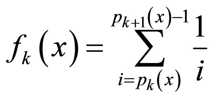
For a base of , consider the function
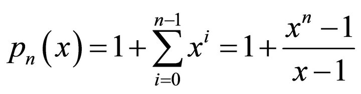
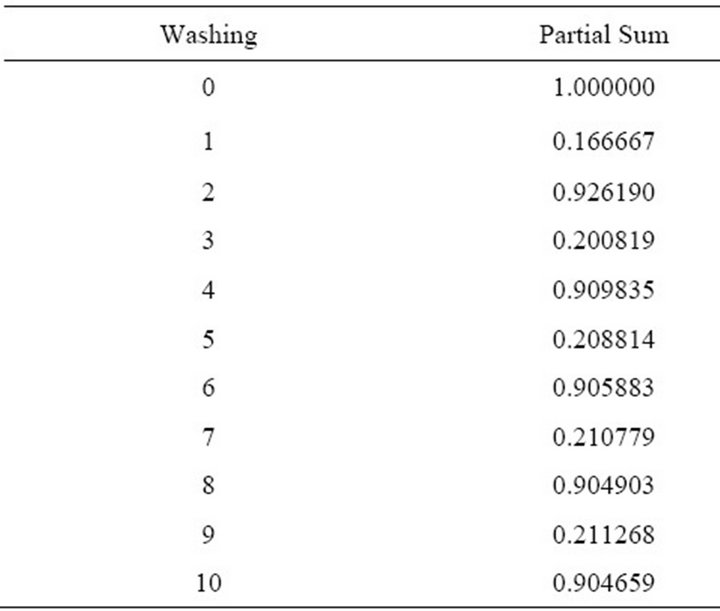
Table 1. Partial sums of washings for base 2.
where the last equality follows from the usual partial sums of a geometric sum (when ) and it is understood that
  is always equal to
  in the case that
 . Then we can express our washing as
and our general positive integer case series as
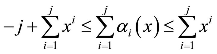
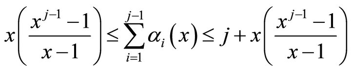
Proposition 3.1. We have ![]()
Proof: The proof of this proposition mirrors the proof of Proposition 2.1 using the fact that
As in Section 2, we indeed obtain a biconvergent series for . We remark that in the case of
 , the number of terms in a washing is always 1 and the series we obtain is the alternating harmonic series which is well-known to converge to
 . The limiting value of
  is actually
  which agrees with the definition of a series converging as opposed to biconverging.
4. The General Case
We now consider the behavior of this process with noninteger bases. First, of course, we need to define a notion of what it means to have a summation involving a non-integer number of terms at each step. We use the case when ![]() as an example. First, we add together
as an example. First, we add together  terms of the harmonic series; this would amount to adding just the first term 1. Next we need to subtract
  terms, meaning two whole terms, and then approximately 71.8% of the next term. That is, we subtract the
![]() , the
, the![]() , and about
, and about . Continuingwe need to add the next
  terms. First we take the remaining 28.2% of the
![]() , leaving about 7.107 terms, so we add 7 whole terms, followed by 10.7% of another. Thus this time we add (approximately)
, leaving about 7.107 terms, so we add 7 whole terms, followed by 10.7% of another. Thus this time we add (approximately)
and the process continues.
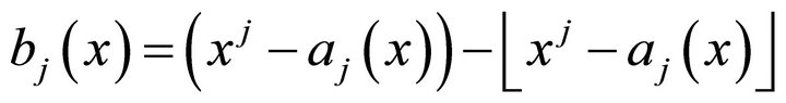
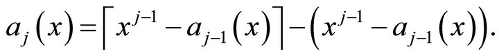
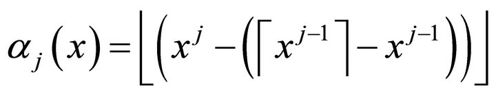
To formalize this process, denote by  and
and  the usual floor and ceiling functions. Define the following functions of
 ![]() and
and  (where
 ![]() is referred to as the base, restricted to
is referred to as the base, restricted to  with
with , and
, and  will be called the washing number):

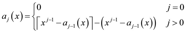


A few remarks are in order. First, note that the definition of  depends on whether or not
 ![]() is an integer. In the
is an integer. In the  case,
case,  and
and  for all
 ; there are no fractional parts of the harmonic series terms to deal with. For this reason,
  is adjusted in these cases to not leave out any harmonic series terms and have
  agree with the washings of Section 3 so that we can define the abstraction of our series from Sections 2 and 3. Now when
 , observe that
  and
and  are the percentages of terms to use in our washing, so these values are between 0 and 1, inclusively. Also, since a term that is only partially added (or subtracted) needs to be completely subtracted (or added) in the next washing, we must have
  . We now prove these statements.
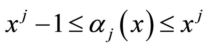
Lemma 4.1. For all x and j, we have  and
and .
.
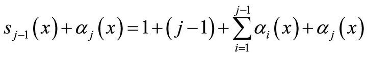
Proof: By definition, when , we have the identity
Let , so that
 , noting then that we must have
 . Similarly, let
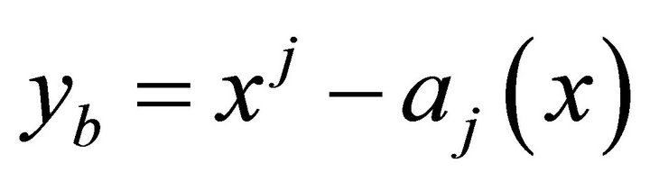 , so that

We then see that  as needed.
Lemma 4.2. For all  and all
 , we have
 .
.
Proof: From the definitions of  and
and , we have

which is equivalent to

Letting , this last equality becomes
 and the proof is complete by noting that
 for any non-integer value of
![]() .
.
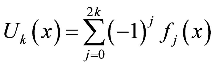
The abstraction of the series in Sections 2 and 3 is given by
which we will call the washed harmonic series of base x. Let us define function  for the upper convergent value of
  and function
  for the lower convergent value of
 . For
. For , denote
and

Also set
![]()
and similarly
![]()
We exhibit in Figure 1 the graphs of  and
and  (the top and bottom “curves” respectively) on the interval
 . The approximations are obtained by using U9(x) and L8(x) on [1,2], U6(x) and L5(x) on
 , and U4(x) and L3(x) on [3,4]; observe that more accurate pictures could be obtained by using many more washings close to 1.
As an interesting note, observe that when![]() , the value of
, the value of  is very close to 0, and the value of
  is very close to 1, giving a possible difference in biconvergent values of
 . Let us formulate and prove the equivalent of Propositions 2.1 and 3.1 in this most general case.
Theorem 4.1. For all x ≥ 1, we have ;
;
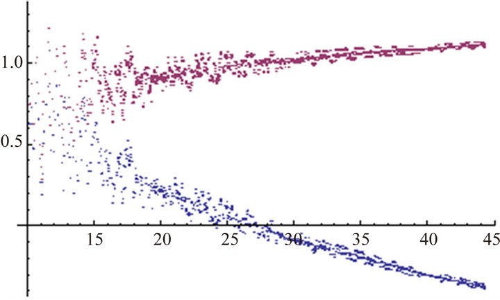
Figure 1. Estimates of upper and lower convergence.
that is, the series biconverges.
Proof: We first consider the definition of  and look at each piece individually. We need not worry about the case when
  to examine the limit as
 . Thus, we have

For (1), from Lemma 4.1, we have  and dividing through by
  produces
Observe that as , we note that
 , thus
  and we can conclude that
The squeeze theorem then yields that the quantity of (1) goes to 0 as . The same reasoning applies to (3) since
  as well. Thus it suffices to consider (2) as the only contributing factor to the limit.
For (2), as with the proof of Proposition 2.1, we use an integral for a lower bound and upper bound on the term. For a fixed , we have
 (4.1)
(4.1)
and
 (4.2)
(4.2)
where  is our variable of integration. The integral in (4.1) we can compute to be
 (4.3)
(4.3)
Note that when ,
,
which is simply

so the inside numerator simplifies nicely. The denominator is simply

When , simply treat the lone j of the numerator and denominator as 0, or appeal to the remark about
  for integer values and Proposition 3.1 for the desired result.
From definition given earlier for the general case of
 , we can quickly observe that since
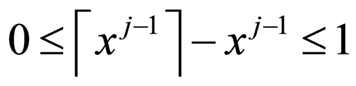 , we must have
 . Thus we also have
or, adding the  from the numerator back and summing the geometric sum,
 (4.4)
(4.4)
Similarly, for the denominator, we will have
 (4.5)
(4.5)
In evaluating the limit on the right-hand side of (4.3), we desire to bound this limit by two others. We can find a lower bound for

by making the numerator as small as possible, and the denominator as large as possible, and we can find an upper bound for it by making the numerator as large as possible and the denominator as small as possible. Using (4.4) and (4.5), we have
 (4.6)
(4.6)
The quantity on the right-hand side of (4.6) can be rewritten as

which goes to  as
as . Examine the inside of the logarithm for the left-hand side of (4.6); its reciprocal can be written as
As , this quantity goes to
 ; thus

as well. The squeeze theorem concludes that the limit in (4.3) is indeed , so
, so
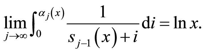
By observing that the integral on the right-hand side of (4.2) can be computed in exactly the same way (adding a 1 to the numerator and denominator of the limit in (4.3) has no effect for the limit), we have
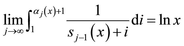
and applying the squeeze theorem gives a limiting value of  to quantity (2) above. Combining (1), (2), and
(3) yields , that is, biconvergence.
5. Analysis
We consider the behavior of our series under different bases as the base ![]() goes to infinity. In Table 2, we give estimates (up to six decimal places) for the integral bases 1 through 10. Note that the case when
goes to infinity. In Table 2, we give estimates (up to six decimal places) for the integral bases 1 through 10. Note that the case when  is again the alternating harmonic series and its upper and lower convergent value is
 . The table includes the various values of
 ,
,  ,
,  and
and . Recall that
  is always equal to
  due to Theorem 4.1.
One observation that could be made from the approximate graphs of  and
and  given in Figure 1 is that both
  and
and  appear unbounded as x goes to infinity. The table above seems to confirm this, but we will now prove the boundedness of
 .
.
Theorem 5.1. The function  is bounded.
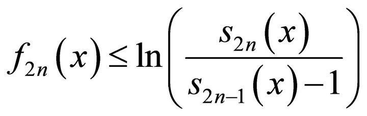
Proof: We prove that  is bounded above first, and proceed accordingly for the lower bound. Recall
 and consider the following grouping:
We use an integral estimate on the value of
 for odd integers
 . To maximize the quantity
 , we wish to minimize

Table 2. Upper and lower convergent estimates.
and maximize . Consequently, for odd
 , since
 and
and , we have that
 , which equals
is greater than or equal to
Evaluating this integral and using the identity  yields
 (5.1)
(5.1)
for integers . Similarly, for even
 , we have that
 , which equals

is less than or equal to
 .
.
This latter quantity is equivalent to
using the facts that 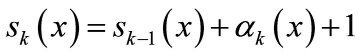 and that
  and
and . Evaluating, we have
 (5.2)
(5.2)
for  Combining (5.1) and (5.2), we have, for
 ,
,

and, in particular, for , we have

when . Using the definition of
 , when
 , we have that

which we can see is
Since the quantity
that appears on the right-hand side is bounded above by 0.25 on the interval , we then have our over-estimate as

which is bounded above on the interval , so U(x) is bounded above, noting that on the interval
  one can show that
  is bounded above by direct computation.
In a very similar fashion, we can obtain a lower estimate by minimizing the quantity . Integral estimates as above yield
for  and
and

when .
.
Similarly, U(x) is then shown to be bounded below by the same process as above, noting that 
is bounded below by −1.2 and  is bounded below by −0.6 on the interval
 . Use the geometric series as above for the other washings for the interval
  and observe that direct computation yields boundedness on
 .
.
As a corollary to Theorem 5.1, we have the following result regarding .
.
Corollary 5.1. The function  is unbounded as
 ![]() goes to infinity.
goes to infinity.
Proof: From Theorem 4.1 before, we know that
 , or, by very quick rearrangement,
 . Given that
  is bounded above and below from Theorem 5.1 and
  is unbounded as
 ![]() goes to infinity,
goes to infinity,  must also be unbounded as
 ![]() goes to infinity.
goes to infinity.
6. Further Questions
There are several natural questions that provide avenues for future work. First, with regards to Theorem 5.1, finding the least upper bound (and greatest lower bound) would be remarkable. Given the behavior of , it seems natural that the lower bound should be when
  (with a value of
 ). A more difficult question is regarding the upper bound; in the proof of Theorem 5.1, the right side of
has a limiting value of  and as
 ![]() goes to infinity, the terms afterwards in
goes to infinity, the terms afterwards in  do not contribute much. We might expect the upper bound to be
 , but computational evidence suggests that
  is never above 1.5, even for large values of
![]() .
.
Another question of interest is that of determining a closed formula for  or
or , or even whether or not one exists. Other natural avenues might examine the properties of
  and
and . Are these functions continuous, or perhaps continuous in a weaker sense? How fast does
  grow, and how fast does
  grow in the negative direction? The presence of the floor and ceiling functions in
  and
and  suggest that
  is not strictly increasing and, in fact, values of
 ![]() can be chosen so that
can be chosen so that  actually decreases slightly on small intervals.
Last, but perhaps certainly not least, what sort of abstraction is there after our most general case? Can we make sense of a three-dimensional model of our “walk across a room”? What other patterns in the number of terms for a washing make sense and are not equivalent to our generalization? With the recent interest in the double, triple, and multiple harmonic series [4-7], how can we apply our methods to those types of series? Is there then a q-series analog or a q-series identity that is a direct result of our methods, similar to [8]?
REFERENCES
- D. Bressoud, “A Radical Approach to Real Analysis,” Mathematical Association of America, Washington DC, 1994.
- L. Zhmud, “Pythagoras as a Mathematician,” Historia Mathematica, Vol. 16, No. 3, 1989, pp. 249-268. doi:10.1016/0315-0860(89)90020-7
- A. Lempner, “A Curious Convergent Series,” The American Mathematical Monthly, Vol. 21, No. 2, 1914, pp. 48-50. doi:10.2307/2972074
- M. Hoffman, “The Algebra of Multiple Harmonic Series,” Journal of Algebra, Vol. 194, No. 2, 1997, pp. 477-495. doi:10.1006/jabr.1997.7127
- M. E. Hoffman and C. Moen, “Sums of Triple Harmonic Series,” Journal of Number Theory, Vol. 60, No. 2, 1996, pp. 329-331. doi:10.1006/jnth.1996.0127
- G. Kawashima, “A Generalization of the Duality for Multiple Harmonic Sums,” Journal of Number Theory, Vol. 130, No. 2, 2010, pp. 347-359. doi:10.1016/j.jnt.2009.03.002
- H. Tsumura, “Multiple Harmonic Series Related to Multiple Euler Numbers,” Journal of Number Theory, Vol. 106, No. 1, 2004, pp. 155-168. doi:10.1016/j.jnt.2003.12.004
- D. Bradley, “Duality for Finite Multiple Harmonic qSeries,” Discrete Mathematics, Vol. 300, No. 1-3, 2005, pp. 44-56. doi:10.1016/j.disc.2005.06.008