World Journal of Mechanics
Vol.07 No.11(2017), Article ID:80697,26 pages
10.4236/wjm.2017.711024
Numerical Simulation of Foaming Processes
Katharina Gladbach1, Antonio Delgado1, Cornelia Rauh1,2
1Institute for Fluid Mechanics, Friedrich-Alexander-University Erlangen-Nuremberg, Erlangen, Germany
2Institute for Food Technology and Food Chemistry, Technical University Berlin, Berlin, Germany

Copyright © 2017 by authors and Scientific Research Publishing Inc.
This work is licensed under the Creative Commons Attribution International License (CC BY 4.0).
http://creativecommons.org/licenses/by/4.0/


Received: November 1, 2017; Accepted: November 26, 2017; Published: November 29, 2017
ABSTRACT
The literature model studied in this article describes bubble formation and growth in a highly viscous polymer liquid with support of a gaseous matter dispersed under pressure before foaming. The foam growth is induced by the application of vacuum and mass transport of volatile components dissolved in the polymer liquid. Based on this literature model, aeration processes are calculated for intermediate viscosity and low viscosity biological systems, as they are of interest for biomatter foams, in particular for food foams in industrial processes. At the end of this article, the numerical results are presented and discussed.
Keywords:
Foaming Process, Conservation Equations, Finite Difference Method, Convergence Analysis, Reynolds Number, Newtonian Liquids

1. Introduction
Foams are of essential importance in nature and in a wide range of technical fields that deal with matter of biological origin such as biotechnology as well as food production and beverage industry. There are several methods to incorporate bubbles within the biomatter structures: mixing, steam generation, gas injection, vacuum expansion and fermentation to name the most important procedures [1] . Recent experimental studies [2] - [7] have established relationships between process parameters and dispersion characteristics. However, there is still a lack of mathematically well-founded physical models that describe bubble formation and behavior in biomatter adequately.
Piesche, Nonnenmacher and Schütz [8] [9] [10] developed models to calculate foaming processes of polymer liquids in a static degassing system, which is supported by a gas dispersed into the polymer liquid under pressure before foaming. The foam growth is induced by a pressure drop and diffusion of volatile components dissolved in the polymer liquid. The related fluid mechanical transport processes are divided into two consecutive models that concern spherical foam and polyhedral foam, respectively. The foam growth is calculated by solving problem-specific conservation equations for mass, momentum and thermal energy. In the present article, the models proposed in [8] [9] [10] are adopted to calculate aeration processes of biomatter. Usually, aeration occurs by applying vacuum or including the gas phase into the liquid phase with a high pressure. Since material parameters for modeling diffusion processes inside biomatter foams do not exist in the literature, they are estimated to illustrate the influence of possible variations.
The model equations [9] are first specified, and the numerical procedures used for solving the model equations in Matlab [11] [12] [13] [14] [15] are outlined. A convergence analysis [16] [17] confirms that the numerical method converges with order 2 in space and at least with order 1 in time. In contrast to the literature [8] [9] [10] , where foaming processes of highly viscous polymer melts are calculated and the Reynolds numbers are Re 1 so that inertia terms in the momentum equation can be neglected [8] (p. 63), foaming processes of food systems [1] - [7] with Reynolds numbers Re ≈ 1 are now calculated. The Reynolds numbers Re ≥ 1 require that inertia terms in the momentum equation have to be taken into account since inertial forces and viscous forces are likewise relevant. At the end of this article, the numerical results are plotted, discussed and compared both with the results presented by Piesche, Nonnenmacher and Schütz [9] [10] for polymer foams and the results given by Haedelt, Beckett and Niranjan [2] [3] for aerated chocolate as a representative of matter of biological origin.
2. Model Equations for Foaming Processes
For the sake of completeness, it is stated that the following considerations postulate physically existent, stable and mathematically unique solutions of the non-linear transport equations for mass, momentum and thermal energy [8] [9] [10] . As mentioned above, mimicking foaming processes occurs by employing two models that describe spherical foam and polyhedral foam, respectively. The model for the spherical foam is based on the assumption that, at the beginning of a foaming process, small monodisperse spherical bubbles are already present in the highly viscous liquid. The bubbles are arranged in a regular cubic spatial structure, see Figure 1 (left). Each elementary cell includes four bubbles, which are composed proportionately. The foam volume of an elementary cell at time t = 0 is given by
, (1)
where cV,0 is the gas volume fraction and rB,0 is the bubble radius before foaming. The gas volume fraction at time t = 0 is given by
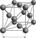
Figure 1. Spherical foam model (left) and growth of a single spherical bubble (right) [9] .
. (2)
The total foam volume Vges,0 at time t = 0 is composed of the gas volume Vg,0 of the bubbles and a liquid volume Vf. The liquid volume that surrounds the bubbles of an elementary cell is constant, regardless of the time:
. (3)
The first model is used to describe the initial phase of foaming until the bubbles begin to influence each other and polyhedral bubbles are formed. In the second model, the monodisperse spherical bubbles are substituted by monodisperse pentagon dodecahedron bubbles. The surface OD and volume VD of a dodecahedron bubble are calculated from the edge length aD of the equilateral pentagon, i.e.
, (4)
. (5)
The constant liquid volume is arranged in a thin layer normal to the surface of the respective bubble. The next three subsections are dedicated to the model equations, which are adopted from the literature [8] [9] [10] .
2.1. Model Equations for the Spherical Foam
The conservation equations for the liquid phase and the transport equations for mass and thermal energy are formulated in spherical coordinates (r, θ, φ). A pure elongational flow is assumed to arise. The velocity of the liquid in radial direction is only relevant and is denoted by u. The velocities in polar and azimuthal direction are zero. Figure 1 (right) illustrates the growth of a single spherical bubble during foaming. At time t = 0, a bubble consists completely of one gaseous matter, for times t > 0, the volatile components dissolved in the liquid diffuse into the bubble. In every time step, the outer radius rS(t) of a constant liquid volume that surrounds the bubble is determined as a function of the current bubble radius rB(t):
. (6)
Equation (6) determines the integration limits for the conservation equations. As shown in [9] , the conservation equation for mass in the liquid phase simplifies to an expression for the radial velocity component (see also Figure 1, right)
. (7)
Similarly, the simplified momentum equation in radial direction r for the single velocity component u is given by
, (8)
where p is the pressure, τrr and τθθ are the normal stresses in radial and polar direction, σ is the interface tension and ρ is the density of the liquid [9] . Inserting the continuity Equation (7) into the momentum Equation (8) and integrating the momentum equation within the limits r = rB(t) and r = rS(t) gives the non-linear, integro-differential equation of motion
(9)
to be solved. Equation (9) assumes that due to the large density differences between the liquid and gaseous phase, no tangential momentum exchange occurs between both phases. The ambient pressure and pressure inside a bubble are interlinked by
, (10)
. (11)
The integral on the right side of Equation (9) characterizes the tensile stresses around the bubble. With regard to the rheological behavior of the liquid, Newtonian, i.e. purely viscous liquids are only considered here. The rheological equation of state for an incompressible Newtonian liquid is S = 2η0D, where S is the extra stress tensor, D is the deformation velocity tensor and η0 is the zero-shear viscosity of the liquid. The normal stress difference in (9) reads then
. (12)
At time t = 0, the temperature ϑ0 and concentrations ξi,0 of the volatile components dissolved in the liquid are postulated to be constant. For t > 0, temperature and concentration profiles arise in the liquid at the phase boundary. The mass transport of the volatile components from the liquid into a bubble is based on the assumptions that the ideal gas law is valid, the components do not influence each other and the concentrations ξi of the components are low so that the Henry law can be applied [9] . Hence, the concentration equation for each component i reads
, (13)
where Di is the diffusion coefficient [9] . Due to the mass transport, a mass balance equation for each component i in the gas phase has to be taken into account [9] :
. (14)
By assuming a homogeneous temperature field inside the bubble, characterized by ϑ(r = rB), the partial pressure pi in the gas phase is calculated by , where Ri and ρi, respectively, are the specific gas constant and the density of the component i. The total pressure pg inside the bubble is the sum of all partial pressures. According to Henry’s law, the concentration of a gas dissolved in a liquid is proportional to the pressure of the respective gas in the gaseous phase. The equilibrium gas concentration and thus the first boundary condition to solve the concentration equation have to be formulated adequately, that is ξGL,i = pi/HW,i, where HW,i is the Henry coefficient of the component i. Due to the mass transport, a transport of thermal energy between the phases also takes place. Further simplified assumptions apply: (i) adiabatic foaming process, (ii) when considering a single bubble, pure one-dimensional heat conduction in radial direction, (iii) negligible production of internal energy by viscous dissipation or diffusion. Under these premises, the transport of thermal energy is expressed by
, (15)
where λW is the heat conductivity and c is the specific thermal capacity of the liquid [9] . Solving the temperature Equation (15) requires knowing the temperature gradient at the phase boundary as the first boundary condition, i.e.
, (16)
where ΔhS,i is the absorption enthalpy of the component i [9] . Equation (16) is completed by work, which is performed to enlarge the bubble surface.
The validity range of the spherical foam model ends if the gas volume fraction exceeds a limit value of about 0.7. In the second model, the bubbles are assumed to have the idealized shape of a pentagon dodecahedron. The transformations at time t*, where the model change occurs, are subject to the following conditions [9] :
(i) The gas volume and liquid volume remain unchanged. (ii) The time derivative of the volume of a bubble is maintained. (iii) The partial pressures in the gaseous phase remain unchanged. (iv) The concentration and temperature profiles are transformed with respect to the constant liquid volume. According to the first condition (i), the edge length aD,begin2 of a pentagon dodecahedron bubble at the beginning of the second model is calculated from the radius rB,end1 of a spherical bubble at the end of the first model:
. (17)
The liquid volume is transformed into a thin layer normal to the bubble surface with thickness
. (18)
The second condition (ii) for the model change leads to the time derivatives
, (19)
. (20)
2.2. Model Equations for the Polyhedral Foam
In the second model, the bubbles are assumed to have the idealized shape of a pentagon dodecahedron. The liquid volume is transformed into a thin layer normal to the surface of the bubbles. According to the model assumption, two neighboring bubbles share a liquid lamella, i.e. the calculations are limited to one half of the liquid lamella. The conservation equations for a liquid lamella are formulated in cylindrical coordinates (r, φ, z) with the velocities u in radial direction and w in axial direction. The geometrical formulation in cylindrical coordinates is based on the assumption that the stress state within a side surface of a pentagon dodecahedron bubble does not differ significantly from the stress state within a circular side surface of same area [9] . Figure 2 depicts schematically a liquid layer with height h(t), which is surrounded by the Plateau edges, the gas phase of a dodecahedron bubble and the liquid layer of the neighboring dodecahedron bubble.
The following additional model assumptions apply: In the selected cylindrical coordinate system, a biaxial elongational flow is formed, where the liquid lamella is shortened in axial direction and stretched in the other two directions. The normal stresses τrr and τφφ have the same size. Interface tension forces do not occur due the negligible curvature of the liquid lamella. Under these premises, the conservation equation for mass for the prevailing two-dimensional velocity field in the liquid phase (u, 0, w) reads (see also Figure 2)

Figure 2. Pentagon dodecahedron bubble model [9] .
(21)
with the elongational rate
. (22)
The momentum equation in axial direction z simplifies to
. (23)
Inserting the relation (22) into the momentum Equation (23) and integrating the momentum equation within the limits z = 0 and z = h(t) gives the equation of motion to be solved. The balance of forces at the phase boundary to the bubble z = h(t) and at the Plateau edges of the liquid lamella z = 0 are taken into account so that
(24)
in accordance to [9] . For a Newtonian liquid with zero-shear viscosity η0, the normal stress difference in (24) reads
. (25)
The assumptions already made in the first model for the mass and energy transport also apply here in the second model [9] . After the transformation , the concentration and mass balance equation for each component i are given by
, (26)
. (27)
The temperature equation and first boundary condition are given by
, (28)
. (29)
2.3. Model Equations in the Dimensionless Form
The model Equations (9)-(16) for the spherical foam are subjected to the Lagrange coordinate transformation and transformed into dimensionless equations [9] . Similarly, the model Equations (24)-(29) for the polyhedral foam are subjected to the Lagrange coordinate transformation and transformed into dimensionless equations [9] . As shown in [9] , the coordinate transformations ensure that the convective terms in the concentration and temperature Equations (13), (15), (26) and (28) are eliminated. From a dimensional analysis, a set of dimensionless π-numbers is obtained:
, (30)
, (31)
. (32)
The index 0 refers in each case to the time point t = 0, whereas the index i refers to a volatile component i dissolved in the liquid. The dimensionless quantities are indicated by the corresponding capital letters.
The relevant quantities are the time , the radius of a spherical bubble , the outer radius of the liquid volume that surrounds a bubble , the transformed spatial coordinate , the normal stresses and , the temperature , the pressure inside a bubble and the ambient pressure . The additional dimensionless quantities used for the polyhedral foam model are the thickness of a liquid lamella , the edge length of a dodecahedron bubble , the transformed spatial coordinate and the corresponding normal stresses and .
The model equations for the spherical and polyhedral foam in the dimensionless form with appropriate initial and boundary conditions [9] [10] are now specified.
Spherical foam:
Equation of motion at the phase boundary
(33)
and , where .
Newtonian liquid
(34)
Concentration equations
(35)
and ,
and .
Mass balance equations
(36)
and .
Temperature equation
(37)
(38)
,
(Equation (38)) and .
The pressure inside a bubble is determined by .
Polyhedral foam:
Equation of motion at the phase boundary
(39)
and .
Newtonian liquid
(40)
Concentration equations
(41)
,
and .
Mass balance equations
(42)
Temperature equation
(43)
(44)
,
(Equation (44)) and .
3. Numerical Method for Solving the Model Equations
The models developed in [9] [10] have been implemented with the software Matlab. The integro-differential Equations (33)-(38) and differential Equations (39)-(44) present two non-linear systems of equations that are treated consecutively. To solve the equations numerically, a finite difference discretization method and a diagonally implicit Runge-Kutta method are applied. The discretized equations are solved separately from each other. The concentration and mass balance equations, the temperature equation and the equation of motion are solved in this order for each model. Since the equations are non-linear and coupled, they have to be solved iteratively in each time step. For the outer iteration process, a Picard iteration method (fixed-point method with successive substitution) is used. In this section, discretization and solution of the integro-differential Equations (33)-(38) in a time step for the first model are explained. The same considerations apply to solving the differential Equations (39)-(44) for the second model numerically.
The concentration and temperature Equations (35) and (37) are parabolic partial differential equations. They are discretized using the finite difference method. As an example, the concentration Equation (35) for a gaseous component i is studied. The diffusion coefficient is assumed to be constant, that is Di = const. Applying the product rule gives the equation
. (45)
Equation (45) is discretized in with and , where discretization is done first in space and then in time. Note that, in the following, the indices n and k refer to discrete points in space and time. Note also that, in section 3 and section 4.1, the constant discretization parameter h denotes the spatial step size, not the thickness of a liquid lamella in the polyhedral foam. With the constant discretization parameter , , the set of all spatial grid points is defined: . The discretization of with the constant discretization parameter h is always equidistant.
The spatial derivatives in (45) are approximated by central difference quotients. Inserting the central difference quotients in (45) gives a coupled system of ordinary differential equations for the unknown functions of the gaseous components dissolved in the liquid, , , that is
(46)
For the time discretization, the grid is selected, where the discretization parameter , , is the temporal step size. The system (46) is integrated by one-step-θ methods [16] [17] . The parameter determines the concrete difference scheme. If the right side of Equation (46) is referred to as , the integration within the limits and gives
(47)
For , the Equations (47) have always accuracy order 2, since RB(Tk + 1) is not known yet and RB(Tk) or an approximated value obtained after an iteration step has to be inserted. The following abbreviations are now defined:
, (48)
, (49)
. (50)
Inserting the expressions for and in (47) gives the discretized equations for the variables , that is
(51)
For each discrete time point Tk, the grid function is defined. The equations for the grid function are obtained when the error term in (51) is omitted:
(52)
Hence, the discrete solution is determined by a linear system of equations
, (53)
,
that has to be solved in each time step. The initial and boundary conditions are taken into account by the vector , the first and the last component of which are only non-zero. The matrix is diagonal if θ = 0 and tridiagonal otherwise. The following one-step-θ methods are often used in practice: explicit Euler method of order 1 (θ = 0), implicit Euler method of order 1 (θ = 1) and, finally, Crank-Nicolson method of order 2 (θ = 0.5) [16] [17] . If Ih is the identity matrix associated with the discretization, the matrix (similarly ) has the form:
(54)
The numerical analysis is based on the properties of M-matrices. In the appendix, relevant definitions and theorems relating to M-matrices [14] [15] [16] [17] are summarized. Since , and is satisfied for all spatial and temporal grid points if in (48)-(50), following properties can be shown:
1) The matrix satisfies the sign condition in definition 1.
2) The matrix is diagonally dominant and irreducible.
According to theorem 1, is regular, according to theorem 2, is even an M-matrix. Hence, the linear system of Equations (53) is uniquely solvable. For a vector , it can be shown that , i.e.
for ,
for ,
for .
Hence, theorem 3 is applicable, and the following estimation is valid:
. (55)
Estimation (55) is relevant for the convergence considerations in the next section. The Equation (46), which is discretized in space, represents a stiff system of ordinary differential equations. The greatest eigenvalue compared to the smallest eigenvalue behaves like O(h−2). Therefore, A-stable numerical time integration procedures are required [16] [17] .
The temperature Equation (37) is discretized and solved similarly to the concentration Equation (35). The mass balance Equation (36) is integrated by the one-step-θ method, which is also used for the concentration Equation (35). The equation of motion (33) is transformed into a system of first order integro-differential equations. Since stiffness occurs, this system is solved by the TR-BDF2 method implemented in Matlab. The TR-BDF2 method is a diagonally implicit Runge-Kutta method of order 2 with associated error estimate of order 3 and is L-stable and also strongly S-stable [11] [12] [13] . For an incompressible Newtonian liquid, the integral in (33) can be calculated analytically so that the system depends only on time (see Equation (34)). The equation of motion (33) requires particularly a high computing time if a low-viscosity Newtonian liquid is given so that a small temporal step size has to be chosen.
4. Presentation and Discussion of Results
4.1. Considerations on Convergence
This section aims at proven convergence of the finite difference discretization method and its order [11] - [17] . The convergence considerations concern the transport processes of mass and thermal energy from the liquid in the gas phase. The convergence theory is based on the properties of the class of M-matrices and follows the numerical studies [16] [17] . It is stated that the outer iteration method gives convergent approximated values. The error function at time Tk is defined by
. (56)
Rh denotes the restriction operator that gives the exact solution of (45) in the spatial grid points at time Tk, whereas is the approximated solution. From (51)-(52), it follows that the finite difference method is consistent. The maximum norm of the local truncation error is
. (57)
Now, the global discretization error is studied. Note that, from (51)-(52), it follows
. (58)
Applying to gives
(59)
Hence, a recursion formula for the error function is obtained. Multiplying Equation (59) from left by the inverse matrix and applying the maximum norm gives
. (60)
By recursive application, the following in equation is obtained:
(61)
The matrix norm of can be determined:
(62)
hence if
(63)
Using (55) and (62) in (61), it follows
(64)
The finite difference method is consistent and stable and thus convergent. The
stability results from the fact that are M-matrices and for
each discrete time point. The convergence analysis also shows that the finite difference method has convergence order 2 in space and at least convergence order 1 in time. Analogous studies can be carried out for the concentration and temperature equations in the second model, where similar results are obtained. In the numerical simulations, the implicit Euler method is used because this method is A-stable and it is not subject to the restriction (63).
4.2. Results of the Numerical Simulations
As a reference example, the foaming process of a two-phase system consisting of polystyrene, styrene and nitrogen is considered. The nitrogen was dispersed into polystyrene under pressure and is in form of small spherical bubbles, but also in dissolved form in polystyrene, whereas styrene is already dissolved in polystyrene. The necessary material and process data are taken from the literature [9] [10] , see Table 1 and Table 2. The time process of the pressure drop is given by
, (65)
where Kexp = 0.6 s−1 is the pressure drop coefficient. The coefficient Kexp is chosen so that the minimal pressure p∞,min = 0.025 bar is reached from the maximal pressure p∞,max = 10 bar after about 10 seconds. The heat conductivity and specific thermal capacity of polystyrene are specified by λW = 0.17 W/(m・K) and c = 1500 J/(kg・K). Note that, at time T = 0, the bubbles consist only of nitrogen. For T > 0, the gaseous components dissolved in polystyrene diffuse into the bubbles.

Table 1. Material data for the system polystyrene/styrene/nitrogen at 240˚C [9] .
Table 2. Process data for the system polystyrene/styrene/nitrogen at 240˚C [9] .
In summary, foam growth is induced by dispersion of nitrogen, vacuum application and diffusion of the volatile components dissolved in polystyrene.
The dimensionless foam volume V is determined on the basis of an elementary cell in the first model (see Equations (1)-(3)), i.e.
, (66)
and on the basis of a single bubble and the constant liquid volume around it in the second model (see Equation (5)), i.e.
. (67)
The local considerations suggest the definition of a local Reynolds number that characterizes the foaming process. The Reynolds number is defined by , where q is the volume flow rate, is the kinematic viscosity and l is the length of the relevant flow region [18] . Selecting the volume flow rate, when the model changes from spherical to polyhedral foam, gives the local Reynolds number
. (68)
The volume flow rate q is determined by the time derivative of the foam volume in Equation (66). The maximal bubble radius can be calculated analytically,
, (69)
and is RB,max = 6.1358 in the examples studied here, whereas the time derivative dRB,max/dT has to be determined by simulation. The constant liquid volume VS surrounds the bubbles of an elementary cell in the first model:
. (70)
If only spherical foam is formed, the volume flow rate q with the maximal time derivative dRB/dT is chosen. In this case, both quantities, the bubble radius RB and its derivative dRB/dT, have to be determined by simulation.
Figure 3 illustrates the simulation results, where polystyrene is assigned a Newtonian rheology. At time T = 0, the gas volume fraction is cV,0 = 0.01, the bubble radius is rB,0 = 100 μm and the initial concentration of nitrogen is ξ1,0 = 0.072%. The initial concentration of nitrogen is chosen so that nitrogen is just in balance. The ambient pressure P∞ decreases exponentially with time according

Figure 3. Bubble radius RB (red) in the first model, lamella thickness H (green) in the second model and foam volume V (blue) as functions of the time T for the two-phase system polystyrene/styrene/nitrogen.
to Equation (65) and is constant after having reached the minimum. In Figure 3 , the bubble radius RB (red), the lamella thickness H (green) and the foam volume V (blue) are plotted as functions of the time T over a period of 60 seconds. As expected, the bubble radius in the first model increases, the lamella thickness in the second model decreases and the foam volume increases continuously until a maximum value is reached. The model change from spherical foam to polyhedral foam is indicated by a point of discontinuity (black dotted line parallel to the y-axis) in the red/green graph. After 60 seconds, the foam volume has reached the maximum value.
In Figure 4, the concentration profiles of nitrogen and the aromatic compound are plotted at different times for the example described above. The concentration profiles are shown as functions of the liquid volume around a bubble. The liquid volume is normalized by the constant liquid volume that surrounds a bubble. At the beginning, nitrogen and the aromatic compound are uniformly dissolved in polystyrene. The partial pressure of nitrogen decreases with the ambient pressure continuously. Hence, the nitrogen concentration decreases quickly at the phase boundary between liquid and gas so that large concentration differences occur in the liquid. Due to the larger diffusion coefficient, nitrogen diffuses anyway faster into the bubbles than the aromatic compound. After 10 seconds, nitrogen is almost completely desorbed. In contrast to nitrogen, the partial pressure of the aromatic compound decreases more slowly. After 60 seconds, finally, the hydrodynamic and thermodynamic equilibrium is reached, i.e. pressure differences between the bubbles and their environment and concentration differences in the liquid are balanced (constant in space and time), see also Table 3.

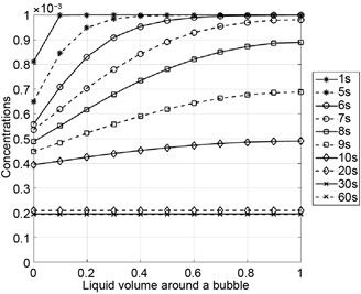
Figure 4. Concentration profiles for nitrogen (left) and styrene (right) as functions of the normalized liquid volume around a bubble for the system polystyrene/styrene/nitrogen.
Table 3. Two-phase system polystyrene/styrene/nitrogen in equilibrium after foaming.
In the following, aeration processes at the temperature 20˚C are calculated for intermediate viscosity and low viscosity systems that are representative for food systems: It is assumed that the liquid has a Newtonian rheology and the density and surface tension of water, i.e. ρ = 1000 kg/m3 and σ = 0.072 N/m, for the purpose of comparison. Nitrogen is dispersed into the liquid under pressure before foaming. First, mass and heat transport are neglected so that the foam growth is induced only by a pressure drop after dispersion of nitrogen. The necessary material and process data are taken from the Table 1, Table 2, unless otherwise specified in this subsection. In contrast to the literature [8] [9] [10] , Newtonian liquids of intermediate or low viscosity are considered. Numerical simulations are carried out for two-phase systems with the viscosity 500 Pas, 50 Pas, 5 Pas, 0.5 Pas, 0.05 Pas and 0.005 Pas, respectively, over a period of 30 seconds. Reynolds numbers Re ≈ 1 require that inertia terms on the left side of the Equations (33) and (39) have to be taken into account. In Figure 5, the
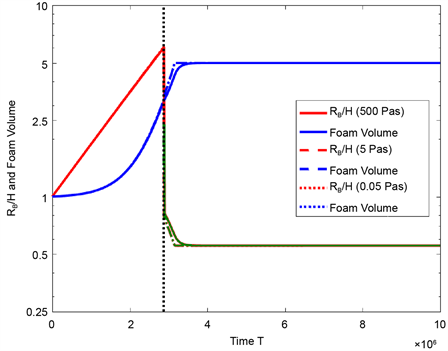
Figure 5. Bubble radius RB (red) in the first model, lamella thickness H (green) in the second model and foam volume V (blue) as functions of the time T for different two-phase systems without mass and heat transport during foaming.
simulation results are plotted for the systems with the viscosity 500 Pas, 5 Pas and 0.05 Pas. It becomes apparent that the two-phase systems behave similarly during foaming and that they attain the same equilibrium state after foaming. The hydrodynamic equilibrium is reached after 10 or 20 seconds. Table 4 specifies the values of relevant material and process quantities after foaming and shows that the less viscous the liquid is, the faster the change from spherical to polyhedral foam occurs.
In addition, aeration processes at the temperature 20˚C are calculated for intermediate viscosity and low viscosity systems, where mass and heat transport from the liquid in the gas phase are included. It is assumed that the liquid has again a Newtonian rheology and the density and surface tension of water, ρ = 1000 kg/m3 and σ = 0.072 N/m. Nitrogen was dispersed under pressure before foaming and is in form of small spherical bubbles, but also in dissolved form in the liquid, whereas a flavoring substance with the properties of styrene is already dissolved in the liquid. Hence, the foam growth is induced by dispersion of nitrogen, vacuum application and diffusion of dissolved components. Since Newtonian liquids of intermediate or low viscosity are considered, inertia terms in the Equations (33) and (39) are taken along. Numerical simulations are carried out for two-phase systems with the viscosity 500 Pas, 50 Pas, 5 Pas, 0.5 Pas, 0.05 Pas and 0.005 Pas, respectively, over a period of 30 seconds, according to the material and process conditions given in the Table 1, Table 2, unless otherwise specified in this subsection. In Figure 6, the simulation results are plotted for the systems with the viscosity 500 Pas, 5 Pas and 0.05 Pas. The same observations
Table 4. Two-phase systems in equilibrium after foaming (without mass and heat transport).

Figure 6. Bubble radius RB (red) in the first model, lamella thickness H (green) in the second model and foam volume V (blue) as functions of the time T for different two-phase systems with mass and heat transport during foaming.
described above can also be made here: The two-phase systems, which differ only in the viscosity of the liquid, behave similarly during foaming and attain the same equilibrium state after foaming. Due to the mass and heat transport, a higher foam volume is reached than in the two-phase systems without diffusion. The concentration profiles of nitrogen and the flavoring substance in Figure 7 confirm that the flavoring substance desorbs faster in a low-viscosity liquid. To clarify the numerical simulation results, Table 5 contains the values of relevant material and process quantities after foaming. The hydrodynamic and thermodynamic equilibrium between the liquid and gas phase is reached after 20 seconds, i.e. pressure differences between the bubbles and their environment and concentration differences in the liquid are balanced.
Table 3 shows that another equilibrium state for the polymer system is reached, which can be explained by the higher temperature 240˚C, compared to the lower temperature 20˚C of the systems characterized in Table 5 after foaming. A local Reynolds number Re ≈ 1 is obtained in each case. Generally, the definition of a global Reynolds number would give values Re ≳ 1 in the Table 4, Table 5.
At the end, the simulation results are compared with the experimental results presented by Haedelt, Beckett and Niranjan [2] [3] . The authors investigated bubble formation in liquid tempered chocolate, which is an example of an intermediate viscosity food system. After the tempering procedure, nitrogen (or another gas) was injected into the chocolate mass under controlled pressure and finely dispersed using a stator and rotor arrangement. When the mixture was returned to atmospheric pressure, the gases dissolved in the chocolate desorbed, and bubbles were formed [2] [3] . The operating conditions were chosen as follows: system pressure p∞,max = 4.5 bar, p∞,min = 1.0 bar, chocolate temperature ϑ0 = 30˚C [3] (p. E139). The remaining data not determined are taken from the Table 1, Table 2, but now pressure drop coefficient Kexp = 0.15 s−1, bubble radius

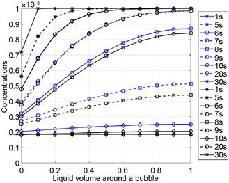
Figure 7. Concentration profiles for nitrogen (left) and a flavoring substance (right) as functions of the normalized liquid volume around a bubble for Newtonian liquids with the viscosity 500 Pas (blue) and 0.05 Pas (black), respectively.
Table 5. Two-phase systems in equilibrium after foaming (with mass and heat transport).
rB,0 = 25 μm and chocolate viscosity η0 = 10 Pas. Furthermore, ρ = 1000 kg/m3 and σ = 0.072 N/m.
The simulations results plotted in Figure 8 over a period of 30 seconds show that a fine spherical foam is obtained. The maximal bubble radius is rB,max = 0.0882 mm, and the gas volume fraction is cV,t = 0.3073 in agreement with the experimental results [3] (p. E141) for aerated chocolate produced by using nitrogen. The low gas volume fraction cV,t is especially a result of the moderate pressures p∞,max and p∞,min chosen, see also Table 6.
The literature model [8] [9] [10] is also applicable if the liquid has a non-Newtonian rheology. The equations of motion (9) and (24) for the spherical and polyhedral foam have to be modified according to the constitutive equation used. In [9] , the rheological behavior of a viscoelastic polymer liquid is described using the generalized contravariant Maxwell-Oldroyd model based on a discrete relaxation time spectrum λR,m and ηm with η0 = Σηm [19] [20] [21] [22] . The simulation results are presented and discussed in [9] [23] [24] and show that the elastic material properties of a viscoelastic liquid do not influence significantly the foaming process under the given conditions. The same equilibrium state is reached, but with delay in time.

Figure 8. Bubble radius RB (red) and foam volume V (blue) as functions of the time T for liqiuid tempered chocolate with dissolved gases.
Table 6. Two-phase system chocolate/flavor additive/nitrogen in equilibrium after foaming.
5. Conclusions
In the present article, aeration processes of intermediate viscosity and low viscosity systems are calculated, based on a literature model. The literature model describes growth of a polymer foam under vacuum with support of a gas dispersed into the polymer liquid before foaming. Numerical simulations are carried out for two-phase systems that are of intermediate or low viscosity and that differ only in the viscosity at a temperature of 20˚C. The necessary material and process data are taken from the literature. Reynolds numbers Re ≈ 1 require that inertia effects in these systems have to be taken into account. The simulations show that the two-phase systems behave similarly during foaming and that they attain the same equilibrium state after foaming. The less viscous the liquid is, the faster the hydrodynamic and thermodynamic equilibrium is reached, i.e. pressure differences between the bubbles and their environment and concentration differences in the liquid are balanced. The numerical method used for solving the model equations was analyzed with respect to stability, consistency and convergence in order to ensure accurate numerical simulation results, which are of interest e.g. for food foams in industrial processes.
Acknowledgements
This research project was supported by the German Ministry of Economics and Technology and the FEI (Forschungskreis der Ernährungsindustrie e.V., Bonn). Project AiF 17125 N. This project is part of the cluster “Proteinschäume in der Lebensmittelproduktion: Mechanismenaufklärung, Modellierung und Simulation” funded by the FEI and the AiF.
Cite this paper
Gladbach, K., Delgado, A. and Rauh, C. (2017) Numerical Simulation of Foaming Processes. World Journal of Mechanics, 7, 297-322. https://doi.org/10.4236/wjm.2017.711024
References
- 1. Campbell, G.M. and Mougeot, E. (1999) Creation and Characterisation of Aerated Food Products. Trends in Food Science & Technology, 10, 283-296. https://doi.org/10.1016/S0924-2244(00)00008-X
- 2. Haedelt, J., Pyle, D.L., Beckett, S.T. and Niranjan, K. (2005) Vacuum-Induced Bubble Formation in Liquid-Tempered Chocolate. Journal of Food Science, 70, E159-E164. https://doi.org/10.1111/j.1365-2621.2005.tb07090.x
- 3. Haedelt, J., Beckett, S.T. and Niranjan, K. (2007) Bubble-Included Chocolate: Relating Structure with Sensory Response. Journal of Food Science, 72, E138-E142. https://doi.org/10.1111/j.1750-3841.2007.00313.x
- 4. Jimenez-Junca, C., Sher, A., Gumy, J.-C. and Niranjan, K. (2015) Production of Milk Foams by Steam Injection: The Effects of Steam Pressure and Nozzle Design. Journal of Food Engineering, 166, 247-254. https://doi.org/10.1016/j.jfoodeng.2015.05.035
- 5. Huppertz, T. (2010) Foaming Properties of Milk. A Review of the Influence of Composition and Processing. International Journal of Dairy Technology, 63, 477-488. https://doi.org/10.1111/j.1471-0307.2010.00629.x
- 6. Kamath, S., Huppertz, T., Houlihan, A.V. and Deeth, H.C. (2008) The Influence of Temperature on the Foaming of Milk. International Dairy Journal, 18, 994-1002. https://doi.org/10.1016/j.idairyj.2008.05.001
- 7. Dickinson, E. (1997) Properties of Emulsions Stabilized with Milk Proteins. Overview of Some Recent Developments. Journal of Dairy Science, 80, 2607-2619. https://doi.org/10.3168/jds.S0022-0302(97)76218-0
- 8. Nonnenmacher, S. (2003) Numerische und experimentelle Untersuchungen zur Restentgasung in statischen Entgasungsapparaten. Dissertation, VDI Verlag Düsseldorf.
- 9. Piesche, M., Nonnenmacher, S. and Schütz, S. (2008) Modelluntersuchungen zur Restentgasung von Kunststoffschmelzen mit gasförmigen Schleppmitteln in einem statischen Entgasungsapparat. 1. Teil: Modellierung des Wachstums eines geschlossenzelligen Polymerschaums. Chemie Ingenieur Technik, 80, 659-675. https://doi.org/10.1002/cite.200700179
- 10. Piesche, M., Nonnenmacher, S. and Schütz, S. (2008) Modelluntersuchungen zur Restentgasung von Kunststoffschmelzen mit gasförmigen Schleppmitteln in einem statischen Entgasungsapparat. 2. Teil: Durchführung und Ergebnisse der Schäumversuche. Chemie Ingenieur Technik, 80, 945-956. https://doi.org/10.1002/cite.200700180
- 11. Alexander, R. (1977) Diagonally Implicit Runge-Kutta Methods for Stiff O.D.E.’s. SIAM Journal on Numerical Analysis, 14, 1006-1021. https://doi.org/10.1137/0714068
- 12. Hosea, M.E. and Shampine, L.F. (1996) Analysis and Implementation of TR-BDF2. Applied Numerical Mathematics, 20, 21-37. https://doi.org/10.1016/0168-9274(95)00115-8
- 13. Prothero, A. and Robinson, A. (1974) On the Stability and Accuracy of One-Step Methods for Solving Stiff Systems of Ordinary Differential Equations. Mathematics of Computation, 28, 145-162. https://doi.org/10.1090/S0025-5718-1974-0331793-2
- 14. Deuflhard, P. and Bornemann, F. (2008) Numerische Mathematik 2. Walter de Gruyter, Berlin, New York.
- 15. Stoer, J. and Bulirsch, R. (2000) Numerische Mathematik 2. Springer-Verlag, Berlin, Heidelberg, New York. https://doi.org/10.1007/978-3-662-09025-1
- 16. Bärwolff, G. (2012) Numerik partieller Differentialgleichungen. Skript. Technische Universität Berlin, Fakultät II: Mathematik und Naturwissenschaften.
- 17. Bastian, P. (2008) Numerische Lösung partieller Differentialgleichungen. Skript. Universität Stuttgart, Fakultät 5: Informatik, Elektrotechnik und Informationstechnik.
- 18. Spurk, J.H. (1992) Dimensionsanalyse in der Strömungsmechanik. Springer-Verlag, Berlin, Heidelberg, New York.
- 19. Oldroyd, J.G. (1953) The Elastic and Viscous Properties of Emulsions and Suspensions. Proceedings of the Royal Society of London A, 218, 122-132. https://doi.org/10.1098/rspa.1953.0092
- 20. Oldroyd, J.G. (1958) Non-Newtonian Effects in Steady Motion of Some Idealized Elastico-Viscous Liquids. Proceedings of the Royal Society of London A, 245, 278-297. https://doi.org/10.1098/rspa.1958.0083
- 21. Böhme, G. (2000) Strömungsmechanik nichtnewtonscher Fluide. Leitfäden der angewandten Mathematik und Mechanik. B. G. Teubner: Stuttgart, Leipzig, Wiesbaden. https://doi.org/10.1007/978-3-322-80140-1
- 22. Giesekus, H. (1994) Phänomenologische Rheologie. Eine Einführung. Springer-Verlag, Berlin, Heidelberg, New York. https://doi.org/10.1007/978-3-642-57953-0
- 23. Gladbach, K., Delgado, A. and Rauh, C. (2014) Modelling and Simulation of the Transport of Protein Foams. Proceedings in Applied Mathematics and Mechanics, 14, 859-860. https://doi.org/10.1002/pamm.201410410
- 24. Gladbach, K., Delgado, A. and Rauh, C. (2016) Modelling and Simulation of Food Foams. Proceedings in Applied Mathematics and Mechanics, 16, 595-596. https://doi.org/10.1002/pamm.201610286
- 25. Walter, W. (2000) Gewöhnliche Differentialgleichungen. Springer-Verlag, Berlin, Heidelberg, New York. https://doi.org/10.1007/978-3-642-57240-1
Appendix
The convergence analysis for the finite difference method in the sections 3 and 4.1 is based on the properties of a special class of matrices, the class of the M-matrices. They are briefly introduced here with reference to the literature [14] [15] [16] [17] [25] . Let be a matrix with the elements and . The set I is called index set. It is written if for all .
In an analogous way, A > B, A ≤ B and A < B. Moreover, 0 denotes the zero matrix.
Definition 1. The matrix A is called M-matrix if
1) for all and for all .
2) A is not singular and A−1 ≥ 0.
Definition 2. with and ⟺ is called graph of the matrix A. If , then i is called directly connected with j. Moreover, i is called connected with j if there is a chain , with for .
Definition 3. A matrix A is called irreducible if each is connected with each .
Definition 4. A matrix A is called diagonally dominant if
for all ,
and irreducibly diagonally dominant if A is irreducible,
for all ,
and the relation < is valid for at least an index .
Theorem 1 [17] . Let be the open circle around
with radius and let be the closed circle.
1) All eigenvalues of A are in
with ,
2) If A is irreducible, the eigenvalues of A are in
.
Theorem 2 [17] . If the matrix A satisfies the sign condition in definition 1 and if A is diagonally dominant or irreducibly diagonally dominant, then, A is an M-matrix.
Theorem 3 [17] . Let A be an M-matrix and let w be a vector with Aw ≥ 1. Then,
.