World Journal of Mechanics
Vol. 1 No. 5 (2011) , Article ID: 8159 , 8 pages DOI:10.4236/wjm.2011.15027
Solution and Type Curve Analysis of Fluid Flow Model for Fractal Reservoir
State Key Laboratory of Reservoir Geology and Exploitation, Southwest Petroleum University, Chengdu, China
E-mail: 373104686@qq.com
Received July 16, 2011; revised August 14, 2011; accepted August 30, 2011
Keywords: Fractal Reservoir, Fractal Dimension, Fractal Index, Type Curve, Well Test
ABSTRACT
Conventional pressure-transient models have been developed under the assumption of homogeneous reservoir. However, core, log and outcrop data indicate this assumption is not realistic in most cases. But in many cases, the homogeneous models are still applied to obtain an effective permeability corresponding to fictitious homogeneous reservoirs. This approach seems reasonable if the permeability variation is sufficiently small. In this paper, fractal dimension and fractal index are introduced into the seepage flow mechanism to establish the fluid flow models in fractal reservoir under three outer-boundary conditions. Exact dimensionless solutions are obtained by using the Laplace transformation assuming the well is producing at a constant rate. Combining the Stehfest’s inversion with the Vongvuthipornchai’s method, the new type curves are obtained. The sensitivities of the curve shape to fractal dimension (θ) and fractal index (d) are analyzed; the curves don’t change too much when θ is a constant and d change. For a closed reservoir, the up-curving has little to do with θ when d is a constant; but when θ is a constant, the slope of the up-curving section almost remains the same, only the pressure at the starting point decreases with the increase of d; and when d = 2 and θ = 0, the solutions and curves become those of the conventional reservoirs, the application of this solution has also been introduced at the end of this paper.
1. Introduction
The concept of fractal geometry, developed by Mandelbort [1], suggests that structures which appear to be completely random can be described within a geometric mathematical framework and offers many possibilities in scientific applications. The class of structures treated in this study is limited to those that exhibit self-similar geometrical properties which mean that the structure looks the same when observed under various scales of measurement. He is also one of the first studiers to find that many structures in nature exhibit these self-similar geometrical properties. Many geological properties affecting the flow of fluids in porous media are known to describe the fractal characteristics.
Hewett [2] reported that porosity and permeability distributions in rock formation demonstrated fractal characteristics and introduced the use of fractal interpolation technique to describe the heterogeneities in a reservoir. Bakker [3] and Doe [4] also developed similar models for the interpretation of constant pressure production/ injection well tests, they both assumed the reservoir properties to vary according to a power law relationship with distance from the source. Chang and Yortsos [5] presented a well testing model which assumed that the fracture network could be described by a fractal distribution. He is also obtained the analytical results, which showed that a fractal reservoir can be identified by a log-log straight line with the slop equals to a function of the fractal dimension and the fractal index. Beier [6] and Aprilian [7] applied fractal reservoir model to analyze well test data for complex reservoirs which could not be matched by traditional model, and the results were consistent with field practice. Poon [8] extended the concept of fractal distribution to study the effect of a composite reservoir. He et al. [9] established a fractal model for unsteady-state flow in dual-porosity and permeability reservoirs based on Warren-Root [10] Model, and solved it by Correction Prediction method. Meanwhile, they analyzed pressure performances and their effect on different factors. Li [11] modified a well test model for infinite dual-porosity reservoir with wellbore storage and skin based on fractal theory, and also resulted a series of applicable analytic solutions. Kong et al. [12] set up equations of flow rate, permeability and porosity for fluid flow in fractal dimensional porous media, and differential equations in different coordinate systems. They solved the model with consideration of wellbore storage and skin, and plotted the solution as type curves. On the basis of Warren-Root mode, Zhang et al. [13], set up a model for deformed dual-porosity fractal gas reservoirs by introducing fractal parameters and compressibility factors. They solved this model by finite element method with consideration of secondary boundary conditions, plotting the results into type curves. To consider threshold pressure gradient in low-perm reservoir and gradual pressure propagation in the formation, Hou and Tong [14] established non-Darcy flow model for deformed dualporosity media. For composite reservoir, there are also many scholars [16-21] have studied it and they also obtained the characteristic curves.
Type curves from models established by above scholars are mainly plotted the pD with tD on bilogarithmic graph, which are greatly different from the traditional ones, and not so applicable in field practice. Therefore, this paper established the flow model for fractal reservoir based on the mechanics of fluid flow in porous media and fractal theory. Analytical solutions are obtained by Laplace transformation and generalized Bessel equation for three kinds of outer-boundary conditions. According to the similar method of Vongvuthipornchai [22] used to plot type curves for non-Newton fluid flow, the corresponding type curves is plotted by Stehfest [23] numerical inversion.
2. Mathematical and Definitions
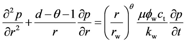
The model was developed with fractured rock in mind, ignored the porosity and permeability of the matrix. The main assumptions of the model include: 1) d-dimensional fractal flowing grids in two-dimensional Euclidean nonpermeable rock, full penetration of the wellbore into reservoir with thickness of h and under radial flow; 2) reservoir fluid is slight-compressive; 3) ignore the effect of gravity and threshold pressure gradient.
According to fractal theory [12], permeability and porosity of the system is:
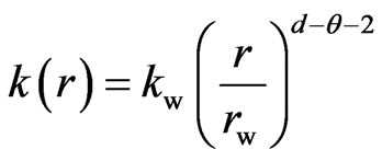 (1)
(1)
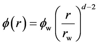 (2)
(2)
Continuity equation for fluid:
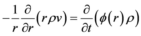 (3)
(3)
Darcy flow equation:
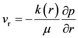 (4)
(4)
Substitution of Equations (1), (2) and (4) into (3):
 (5)
(5)
where: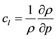 ,
, ,
, .
.
3. Model Solutions
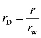
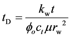
Introducing the following dimensionless variables:
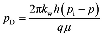 (6)
(6)
 (7)
(7)
 (8)
(8)
Allows the continuity equation to be written in dimensionless terms and consider the boundary and initial conditions, then
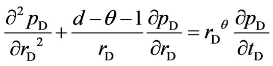 (9)
(9)
The initial pressure distribution is assumed uniform, everywhere
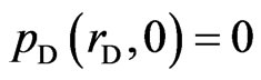 (10)
(10)
Inner boundary conditions
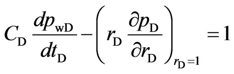
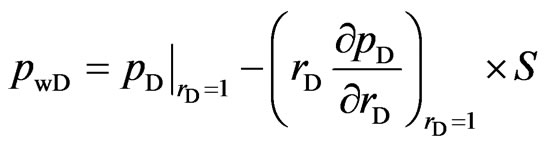 (11)
(11)
 (12)
(12)
And the outer boundary conditions are as follows:
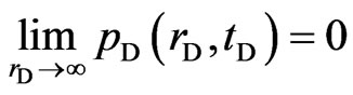 (Infinite reservoir)(13)
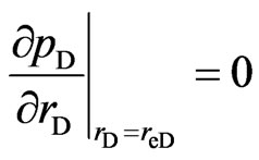 (Closed circle reservoir)(14)
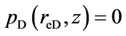
(Circle reservoir with constant-pressure boundary)(15)
To simplify, Equations (9)-(15) are transformed into Laplace space.
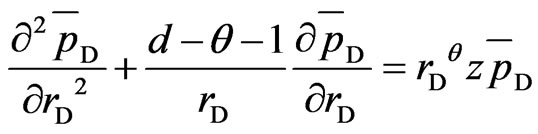 (16)
(16)
where: 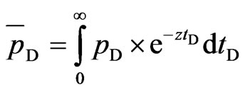
Inner boundary conditions:
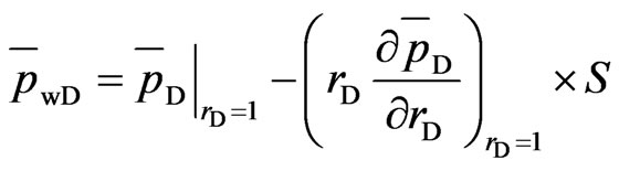 (17)
(17)
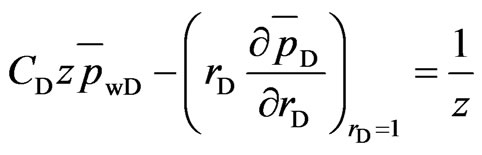 (18)
(18)
Outer boundary conditions:
Infinite reservoir
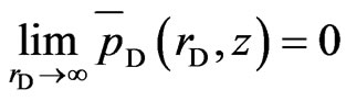 (19)
(19)
Closed circle reservoir
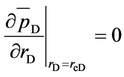 (20)
(20)
Circle reservoir with constant-pressure boundary
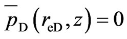 (21)
(21)
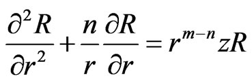
Equation (13) can be solved according to the theory of generalized Bessel equation. Let, 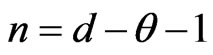 to convert Equation (13) into the format of generalized Bessel equation
 (22)
(22)
where: m = d − 1.
Combining m with n, we have m − n = θ and θ is a constant. Because of 2 + m − n = 2 + θ > 0, and using the method of Bessel function [12], a solution of Equation (16) is assumed in the form:
 (23)
(23)
where: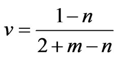 .
.
Define β by:
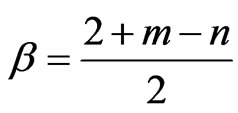 (24)
(24)
Equation (23) reduce to:
 (25)
(25)
Using the method of modified Bessel function [12], the derivative of Equation (25) is:
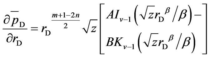 (26)
(26)
Combine Equations (25) and (26) with (17) and (18):
 (27)
(27)
 (28)
(28)
3.1. For Infinite Reservoir
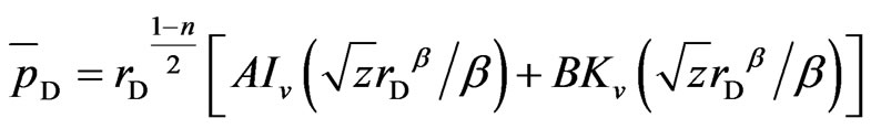
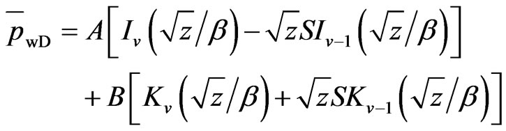
According to the characteristics of Modified Bessel Function [12], as the dimensionless radius approaches infinity Iv becomes infinity; therefore to satisfy the outer boundary condition the constant A must be zero. To determine the constant B, apply the inner boundary condition (Equations (22)-(23)) to Equations (27)-(28). The resulting solution of normalized bottom-hole pressure is the follows:
 (29)
(29)
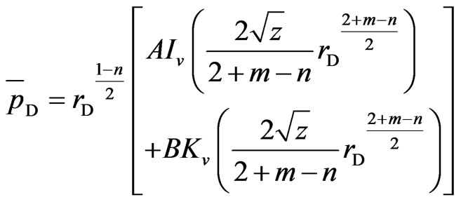
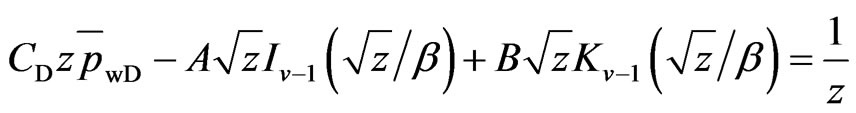
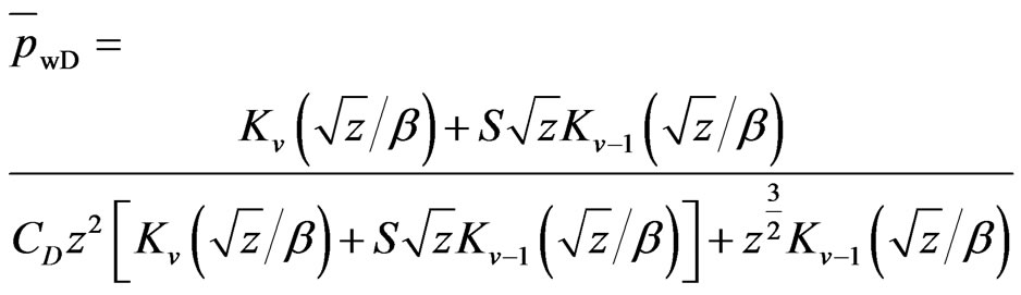
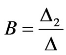
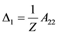
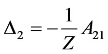
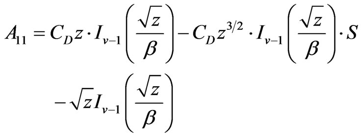
3.2. For Closed Circle Reservoir or Constant-Pressure Boundary Reservoir
Applying the similar method of infinite reservoir, we can obtain the following solution:
 (30)
(30)
where: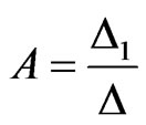 ,
,  ,
, 
 ,
, 
For closed circle reservoir:
For circle reservoir with constant-pressure boundary:

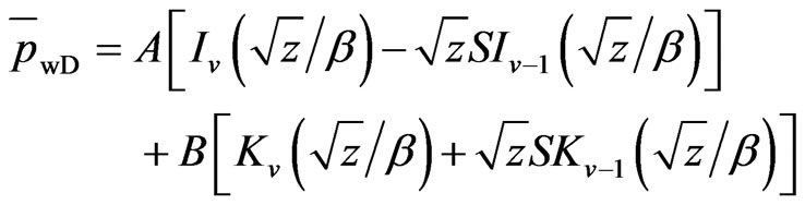
4. Type Curves and Flow Period Analysis
Using the method of Vongvuthipornchai [19], analytical solutions abstained above can be plotted as type curves in bilogarithmic coordinate system with [tD/CD](4-d+θ)/2 as x axis and [pD/CD](2-d+θ)/2, p’D*[tD/CD](4-d+θ)/2 as y axis.
The type curves of infinite fractal reservoir are shown in Figures 1 and 2, Figures 3 and 4 are for closed circle reservoir and circle reservoir with constant-pressure boundary, respectively. According to the type curves, the following flow periods are obtained:
Stage I is the wellbore storage flow period, which is characterized by a unit slop line and not affected by frac-
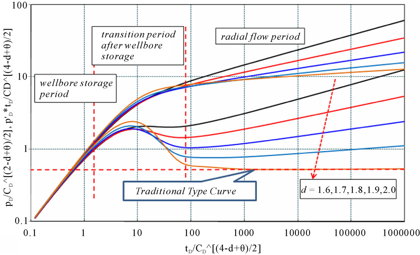
Figure 1. Type curves of infinite reservoir with different fractal dimension d (CD = 1000, S = 2, θ = 0.01).
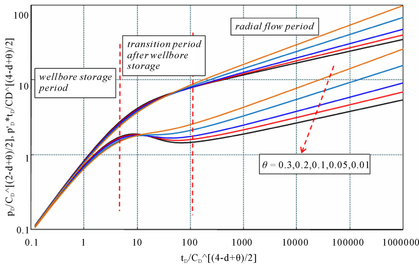
Figure 2. Type curves of infinite reservoir with different fractal factor θ (CD = 1000, S = 2, d = 1.7).
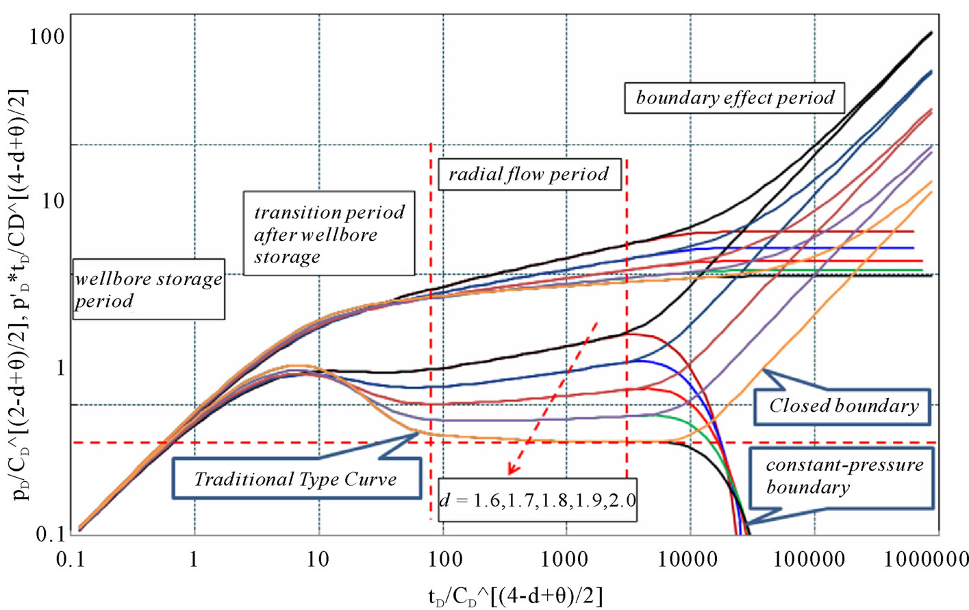
Figure 3. Type curves of closed and constant-pressure boundary reservoir with different fractal dimension d (CD = 100, S = 2, θ = 0.01, reD = 2000).
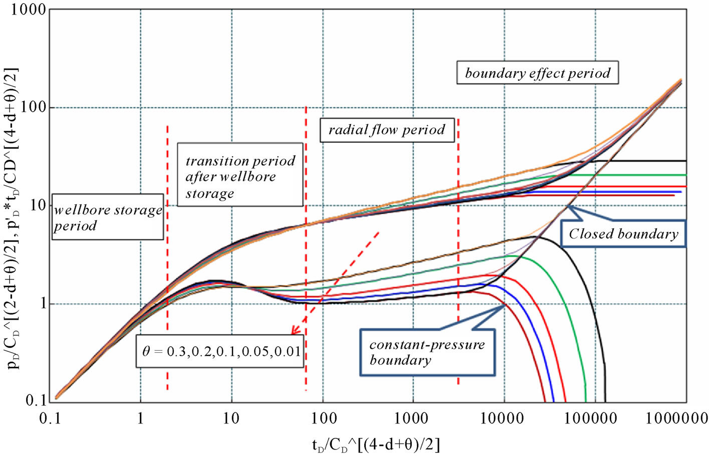
Figure 4. Type curves of closed and constant-pressure boundary reservoir with different fractal factor θ (CD = 100, S = 2, d = 1.8, reD = 2000).
tal dimension d and factor θ.
Stage II is the transition flow period after wellbore storage. Based on the type curves, length and peak value of this period are controlled by wellbore storage effect, skin, d and θ. For a constant θ value, length and peak value decrease with the increase of d; when d is constant, they decrease with θ. According to Figures 3 and 4, the transition period becomes shorter and shorter when d decreases or θ increases.
Stage III stands for radial flow period. For fractal reservoir, it can be noticed from the curves that the radial flow period is no longer a 0.5 straight line as traditional type curves. They become a group of upwards straight lines, whose slopes and starting points are related to d and θ. For constant d and θ, the slope is also a constant with different starting points and pressure (pressure derivative) values.
Stage Ⅳ represents the boundary effect. When the reservoir is infinite, this period will not exit. For closed or constant-pressure boundary reservoir, rapid upor down-curving can be seen on the type curves (see Figures 3 and 4). Closer the boundary is, earlier this change happens, vice versa. According to Figures 3 and 4, for constant-pressure boundary reservoir, when d is fixed, the down-curving happens earlier with θ becoming smaller; and when θ is a constant, the curves do not change too much when d changes. For closed reservoir, when d is a constant, the up-curving has little to do with θ; and when θ is fixed, the slope of the up-curving section is almost a constant, only the pressure at starting point decreases with increase of d.
When d = 2 and θ = 0, the results become the conventional reservoirs’ solutions, and the type curves become the corresponding ones, which are shown in Figure 5. It can conclude that the conventional reservoirs are the special form of fractal reservoirs.
5. Application
A pressure buildup test in an oil well is influenced by skin and wellbore storage. The measured pressure date as a function of time is listed in page 294 of the Bourdet (radial flow example) [11]. And the other known reservoir and well data as follows:
∅ = 0.25, rw = 0.088392 (m), Ct = 0.000609 (MPa−1), h = 32.956 (m), Bo = 1.06 (m3/sm3), μ0 = 2.5 (cp).
A log-log plot (full test history ∆t with pressure and pressure derivative functions) and final match of this example is shown in Figure 6.
Dates are matched against the conventional reservoir type curves for a well with wellbore storage and skin in a reservoir with homogeneous behavior. The property of match type curve is CD = 800, and the S = 7.6. So, from the definition of CD, we have C = 0.2 E − 3 (m3/MPa), and the K∙h = 359 (mD∙m), and so, the effective permeability is 10.89 (mD), which the results obtained are consistent with reference [11].
6. Conclusions
Based on mechanism of fluid flow in porous media and the fractal theory, a model with fractal characteristics for fractal reservoir is constructed and solved by Stehfest’s [20] inversion method. A new method to plot type curves of fractal networks with fractal characteristics was developed. These new type curves have the similar characteristics as those of the conventional ones. Compared to the previous fractal reservoir curves, the improvement is valuable.
Type curves for fractal reservoir are greatly affected by dimension d and factor θ, especially during the radial flow period, where the pressure derivative is not a 0.5 straight line any more, and the slop of the line increases with the decrease of d and increase of θ. During the wellbore storage and boundary flow period the curves have the similar characteristics as conventional reservoir, and when d = 2 and θ = 0, the solutions and curves become those of the conventional reservoir, the example is also supplied during the application when d = 2 and θ = 0, which is a special condition of the fractal reservoir.
7. Acknowledgements
This work was supported by National Program on Key Basic Research Project (973 Program, Grant No. 2011CB201005), Research Fund for the Doctoral Program of Higher Education of China (Grant No. 201051 21110006).

Figure 5. Type curves of infinite reservoir with the (d = 2, θ = 0, S = 2).
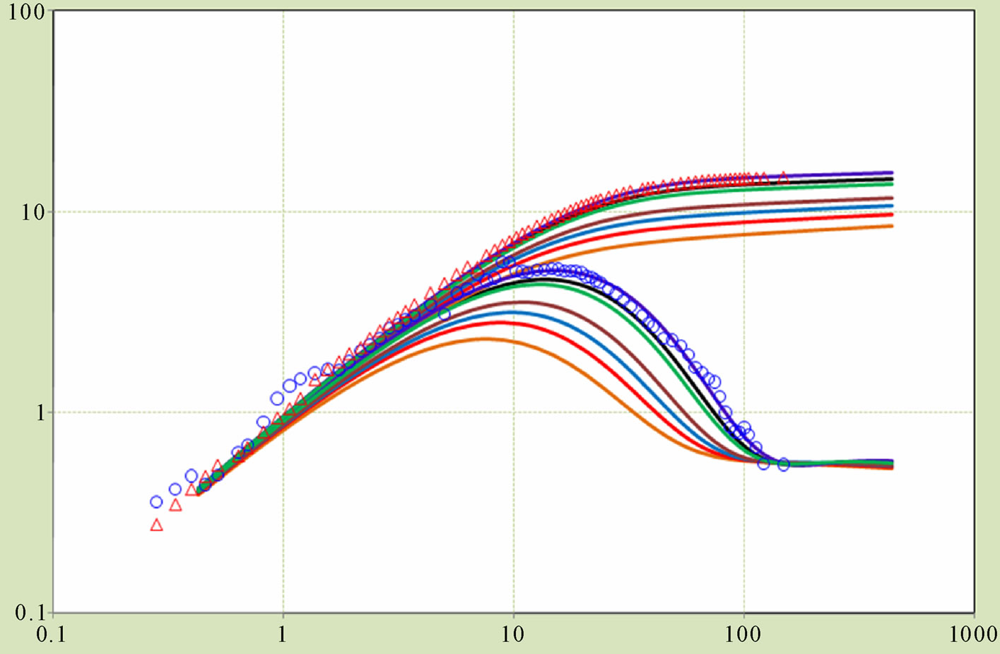
Figure 6. The log-log matching plot.
REFERENCES
- B. B. Mandebort, “The Fractal Geometry of Nature,” W. H. Freeman, New York, 1982.
- T. A. Hewett, “Fractal Distribution of Reservoir Heterogeneity and Their Influence on Fluid Transport,” Society of Petroleum Engineers, New Orlean, 5-8 October 1986, Document ID: 15386.
- J. A. Bakker, “A Generalized Radial Flow Model for Hydraulic Tests in Fractured Rock,” Water Resources Research, Vol. 20, No. 10, 1986, pp. 1796-1840.
- T. W. Doe, “Fractional Dimension Analysis of Constant Pressure Well Tests,” The 66th Annual Technical Conference and Exhibition of SPE, Dallas, 6-9 October 1991. Document ID: 22702-MS. doi:10.2118/22702-MS
- J. Chang and Y. C. Yortsos, “Pressure Transient Analysis of Fractal Reservoir,” SPE Formation Evaluation, Vol. 5, No. 1, 1990, pp. 31-38. doi:10.2118/18170-PA
- R. A. Beier, “Pressure Transient Field Data Showing Fractal Reservoir Structure,” International Technical Meeting of the SPE, Calgary, 10-13 June 1990, Document ID: 21553-MS.
- S. Aprilian, D. Abdassah, L. Mucharant, et al., “Application of Fractal Reservoir Mode for Interference Test Analysis in Kamojiang Geothermal Field (Indonesia),” The 68th SPE Annual Technical Conference and Exhibition, Houston, 3-6 October 1993, Document ID: 26465- MS. doi:10.2118/26465-MS
- D. Poon, “Transient Pressure Analysis of Fractal Reservoirs. The Petroleum Society of CIM,” The 46th Annual Technical Meeting of the Petroleum Society of CIM, Calgary, 7-9 June 1995, Document ID: 95-34.
- G. L. He and K. L. Xiang, “Mathematical Model and Character of Pressure Transient of Unstable Seepage Flow in Deformation Dual-Porosity Fractal Reservoirs,” Journal of Southwest Petroleum University, Vol. 24, No. 4, 2002, pp. 24-28. (in Chinese)
- J. E. Warrant and P. J. Root, “The Behavior of Naturally Fractured Reservoirs,” SPE Journal, Vol. 3, No. 3, 1963, pp. 245-255.
- D. P. Bourdet, J. A. Ayoub and Y. M. Pirard, “Use of Pressure Derivative in Well Test Interpretation,” SPE Formation Evaluation, Vol. 4, No. 2, 1989, pp. 293-302.
- S. C. Li, “A Solution of Fractal Dual Porosity Reservoir Model in Well Testing Analysis,” Progress in Exploration Geophysics, Vol. 25, No. 5, 2002, pp. 60-62. (in Chinese)
- X. Y. Kong, “Advanced Mechanics of Fluids in Porous Media,” University of Science and Technology of China Press, Hefei, 1999. (in Chinese)
- L. H. Zhang, J. L. Zhang and B. Q. Xu, “A Nonlinear Seepage Flow Model for Deformable Double Media Fractal Gas Reservoirs,” Chinese Journal of Conputational Physics, Vol. 24, No. 1, 2007, pp. 90-94. (in Chinese)
- Y. M. Hou and D. K. Tong, “Non-Steady Flow of Non-Newtonian Power-Low Permeability with MovingBoundary in Double Porous Media and Fractal Reservoir,” Engineering Mechanics, Vol. 26, No. 8, 2009, pp. 245-250. (in Chinese)
- K. L. Xiang and X. Q. Tu, “The Analytical Solutions of Mathematical Model for a Fractal Composite Reservoir with Non-Newtonian Power Low Fluids Flow,” Chinese Journal of Computational Physics, Vol. 21, No. 6, 2004, pp. 558-564. (in Chinese)
- X. R. Deng and S. C. Li, “Solution to the Well Testing Model for Fractal Composite Reservoirs,” Journal of Xihua University Natural Science, Vol. 24, No. 2, 2005, pp. 4-7. (in Chinese)
- C. X. Xu, S. C. Li and W. B. Zhu, “Similar Structure of Well Test Analytical Solution in the Fractal Composite Reservoir,” Drilling Production Technology, Vol. 29, No. 5, 2006, pp. 39-43. (in Chinese)
- C. S. Chakrabarty, M. Farouqali and W. S. Tortlke, “Transient Flow Behavior of Non-Newtonian Power-Law Fluids in Fractal Reservoirs,” Annual Technical Meeting of the Petroleum Society of CIM, Calgary, 1993, Document ID: CIM93-06.
- R. R. Dyah, J. C. Kana, A. Doddy, et al., “A New Numerically Model of Single Well Radial Multiphase Flow in Naturally Fracture Reservoir System-Using Fractal Concept,” Society of Petroleum Engineers, 1999, Document ID: 57276.
- X. Y. Kong, D. L. Li and D. T. Lu, “Basic Formulas of Fractal Seepage and Type-Curves of Fractal Reservoirs,” Journal of Xi’an Petroleum University, Vol. 22, No. 2, 2007, pp. 1-5. (in Chinese)
- S. Vongvuthipornchai and R. Raghavan, “Well Test Analysis of Date Dominated by Storage and Skin: Nonnewtonian Power-Law Fluid,” Society of Petroleum Engineers, 1987, Document ID: 14454.
- H. Stehfest, “Numerical Inversion of Laplace Transforms,” Communications ACM, Vol. 13, No. 1, 1970, pp. 47-48.
Nomenclatures
h = reservoir thickness, cm
d = fractal dimension
θ = fractal factor
k = permeability, D
r = radius, cm
v = velocity, cm/s
p = reservoir pressure, atm
t = production time, s
q = production rate, cm3/s
z = Laplace variable
Iv, Kv = modified Bessel function
Greek Symbols
μ = viscosity, cp
ρ = density, g/cm3
∅ = porosity, fraction
Subscripts
D = dimensionless
w = wellbore hole
i = initial
f = fluid
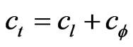
t = total
wD = wellbore dimensionless
eD = external dimensionless