International Journal of Astronomy and Astrophysics
Vol.1 No.2(2011), Article ID:5680,10 pages DOI:10.4236/ijaa.2011.12004
The Relief of Plasma Pressure and Generation of Field-Aligned Currents in the Magnetosphere
Institute of Solar-Terrestrial Physics, Siberian Branch of the Russian Academy of Sciences, Irkutsk, Russia
E-mail: pvlsd@iszf.irk.ru
Received January 31, 2011; revised March 12, 2011; accepted March 28, 2011
Keywords: Magnetosphere, Plasma Convection, Plasma Pressure, Field-Aligned Currents
Abstract
A combined action of plasma convection and pitch-angle diffusion of electrons and protons leads to the formation of plasma pressure distribution in the magnetosphere on the night side, and, as it is known, steady electric bulk currents are connected to distribution of gas pressure. The divergence of these bulk currents brings about a spatial distribution of field-aligned currents, i.e. magnetospheric sources of ionospheric current. The projection (mapping) of the plasma pressure relief onto the ionosphere corresponds to the form and position of the auroral oval. This projection, like the real oval, executes a motion with a change of the convection electric field, and expands with an enhancement of the field. Knowing the distribution (3D) of the plasma pressure we can determine the places of MHD-compressor and MHD-generators location in the magnetosphere. Unfortunately, direct observations of plasma distribution in the magnetosphere are faced with large difficulties, because pressure must be known everywhere in the plasma sheet at high resolution, which in situ satellites have been unable to provide. Modeling of distribution of plasma pressure (on ~ 3-12 Re) is very important, because the data from multisatellite magnetospheric missions for these purposes would be a very expensive project.
1. Introduction
The ionosphere is the ohmic environment where the electric field and current are related by the Ohm’s law. Since the mean free path in the magnetosphere during pair collisions with a Coulomb interaction considerably exceeds the extents of the magnetosphere, it is customary to assume that the magnetospheric plasma is collisionless. A direct relation between the electric field and current is absent in the magnetosphere. Since the geomagnetic field lines are equipotential, the currents in the ionosphere and magnetosphere depend on the magnetospheric electric field and gas pressure distribution, respectively. If the ionospheric current was a purely Hall current, this would not be a dangerous phenomenon since the Hall current is nondivergent and does not deliver a work. In reality, the ionospheric current is combined and always includes the Pedersen component, and the ionosphere is a real energy consumer. Combined actions of some processes in the geomagnetosphere result in the formation of a spatial distribution of gas pressure, i.e., bulk currents in the magnetosphere. Divergence of these bulk currents produces the spatial distribution of field-aligned currents. Thus, the problem of formation of a spatial distribution of plasma pressure in the magnetosphere is still very important. A lot of papers are devoted to this problem, e.g. [1-5].
The goal of our paper is a development of Kennel’s idea [6] and the approach [7,8].
2. Calculation of Plasma Pressure Distribution in the Magnetosphere
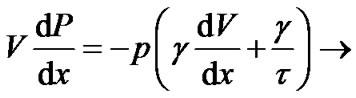
The equations of the two-fluid or one-fluid magnetohydrodynamics with isotropic or anisotropic pressure are as a rule used to describe magnetospheric plasma. In this case any dissipative processes in the system are considered inessential. This statement is usually valid for ohmic loss and loss by radiation. However, particles (and energy) also escape from the magnetospheric plasma into the atmosphere through open ends of flux tubes. This type of loss can be very substantial and should be taken into account. The first consequences of such loss were studied by Kennel [6]. We present the set of equations describing the magnetospheric plasma [7, 8]:
 ,
,
 (1)
(1)
 ;
;
 (2)
(2)
 ;
;
 (3)
(3)
 ;
; 
(4)
Here i = e, p is the index of electrons or protons; ni is the particle number density; pi is the pressure of given particles; t is the current time; U is the plasma tube volume (by plasma tube we mean the plasma content of a magnetic flux tube); E is the electric field strength; B is the magnetic field strength; Vi is the electric drift velocity of the corresponding plasma component; V = Ve + Vp is the drift velocity of plasma as a whole; and j is the electric current density; g = 5/3 – is the adiabatic exponent. If j/en<<V, a difference in the drift velocities between the electron and proton components can be neglected. Hereafter, we will do so if no special assumptions are made. The condition of quasineutrality, i.e., (np – ne)/(np + ne) <<1, is satisfied throughout the magnetospheric plasma. The first equation in the set is the continuity equation for electrons and ions taking into account particle loss due to pitch-angle diffusion into the loss cone. The characteristic time t is the time over which the plasma tube loses 1/e part of the initial number of particles. Equations (2) describe the electron and proton gas pressure behavior during motion due to precipitation. The gas behavior is evidently nonadiabatic. Equations (3) are factually the equations of plasma motion in a quasistationary case. The first equation in (4) is the expression for entropy density. Here cv is heat capacity at a constant volume. Entropy evidently increases in the course of time, and the process of plasma convection is irreversible in our approximation. The second expressions in (1) and (2) are the solutions to the corresponding equations. Our set of magnetohydrodynamic equations was substantiated in detail in [7,8]. The applicability of this set was analyzedand the definitions of t were given in the same work.
From the balance equation of gas kinetic energy in a steady-state one-dimensional case we can obtain:


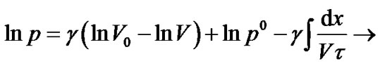
The process of magnetic flux tube depletion due to particle escape into the loss cone is superposed on the above process; then, the gas pressure (for particles 5 - 25 keV) is defined as [7]:

It is evident that dt =dR/VR =R0dl/Vl , Δt = ∫dt is the transport time, i.e., the time over which the flux tube will move from the boundary to the given point on the flux line; and VR and Vl are the radial and azimuthal components of convection velocity. Thus, the expression for pg indicates how gas pressure changes when plasma moves along the convection line at a velocity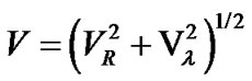 .
.
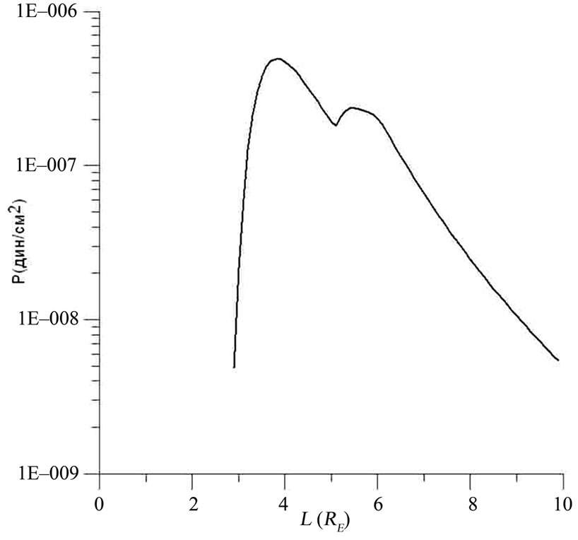
Specifying the initial pressure p0 at the boundary L = L∞, we can find the resultant pressure at any point on the flux line. In such a way, the field of pressures in the entire magnetosphere is calculated (Figures 1 and 2). The magnetic field for these calculations is dipole, and the electric field described in detail in [8].
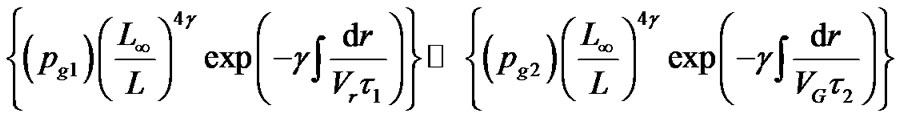
Similarly, it is possible to obtain the following expression (Vr ~20 - 30 km/s; VG ~hundreds of km/s) (Equation.)
This is more exact expression for gas pressure in the magnetosphere on the night side, which takes into account particles with energy up to 300 keV. However, according to estimations and data of satellite measurements (Equation).

1-30 keV 30-300 keV
1 - 30 keV 30 - 300 keV
 (a)
(a)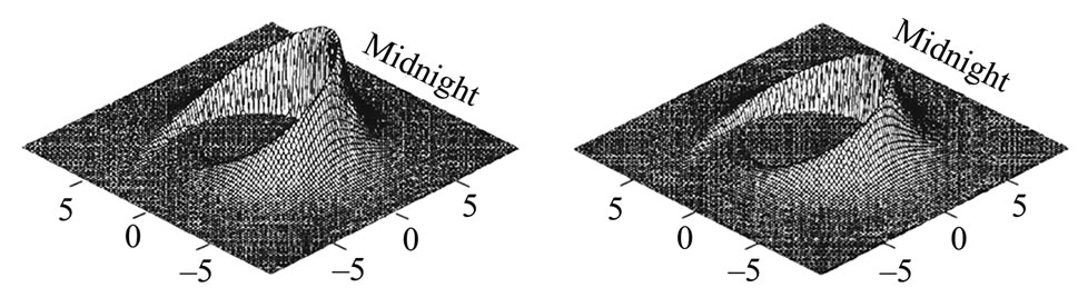 (b)
(b)
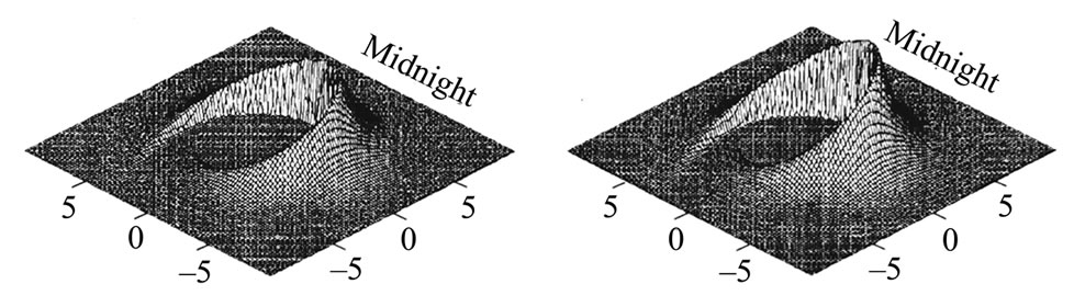
Figure 1. Gas pressure relief under the stationary boundary conditions but with the electric field variable in time: (a) t = 0 s, (b) t = 1000 s, (c) t = 2800 s, and (d) t = 4500 s. The projection (mapping) of the plasma pressure “hump” onto the ionosphere corresponds to the form and position of the auroral oval. This projection, like the real oval, executes a motion with a change of the convection electric field, and expands with an enhancement of the field.

Particles with energy of 5 - 50 keV (mostly, protons) give the greatest contribution to formation of a relief of plasma pressure in the magnetosphere on the night side (~4 - 10 RE), and, as it is known, steady bulk currents are connected to distribution gas pressure. The divergence of these bulk currents brings about a spatial distribution of field-aligned currents, i.e. magnetospheric sources of ionospheric current systems.
Several characteristic details are observed when we consider this three-dimensional plot. First of all, this is the general shape resembling amphitheatre. The crest maximal height is almost at the zero meridian, and the amplitude decreases in both opposite directions. The amphitheatre represents an oval, the contour of which maximally approaches the center from the inside. It is clear that this figure will resemble the auroral oval in the projection onto the ionosphere. The situation changes principally when the boundary conditions are dependent on time (Figures 3 and 4). The solution structure is so that p0(t) can be considered as an input signal multiplied by the transfer function p(t`) = G(t) A(L):
 ;
;

The projection (mapping) of the plasma pressure “hump” onto the ionosphere corresponds to the form and position of the auroral oval. This projection, like the real oval, executes a motion with a change of the convection electric field, and expands with an enhancement of the field. The flux density of precipitating electrons at the level of the ionosphere will be [7,8]:
j׀׀е = BIòndl/Bt The time variation in precipitation during a model substorm is shown in Figure 5.
3. Computation of Field-Aligned Currents
The plasma movement equation in the single-liquid approximation:
 where V – is the mass movement velocity, r – plasma density, р – gas pressure, j – current density, B – magnetic field intensity. Having multiplied the equation on V and taking into account that we can always neglect the inertia power in magnetosphere, we get a very important for the Earth magnetosphere physics ratio [7]: VÑp = Ej. In the left part of it we have the hydrodynamic quantities, and in the right one—electrodynamic ones. The physical sense of this equation is clear. If the gas is moving to the pressure increase (i.e. in the plasma coordinate system happens its compression—the compressor «works»), then Ej > 0. Now we have the consumer of the electric power – MHD compressor. If the plasma is flowing to the side of pressure decrease, then the gas-kinetic power can provide a work over the electric ones. Knowing the propagation of the plasma pressure we can determine the places of MHD-compressor and MHD-generators location in the magnetosphere (Figure 7; see in details [7,8]). The generators feed the current systems of BirkelandBostrom (BB) of the first and second types [9,10].
 (a)
(a)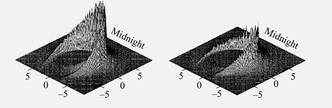 (b)
(b)
Figure 3. Gas pressure relief (results of the modeling) under the nonstationary boundary conditions: (a) t = 0 s, (b) t = 1000 s, (c) t = 2800 s, and (d) t = 4500 s.
 (a)
(a) (b)
(b)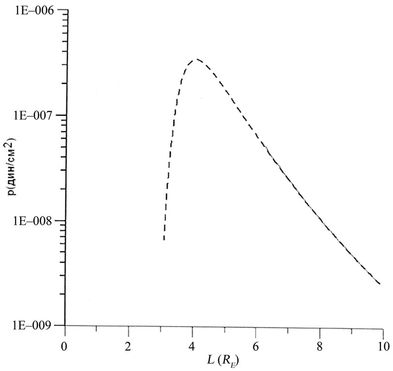 (c)
(c)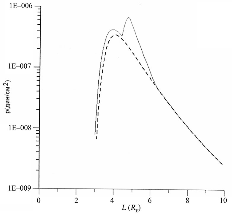 (d)
(d)The second amphitheatre and a specific corridor between the amphitheatre and the main crest appear in Figure 3(b). The cross section of this spatial pattern along any intermediate contour line is shown in Figure 8. Figure 8 indicates that the field-aligned currents are directed oppositely on both sides of the corridor. Since the sign of the pg gradient changed and that of the pB gradient remained unchanged, the double “curtain” of field-aligned currents is formed, which is a characteristic feature of auroral electrojet feeding [11]. The geometry of these electrojets corresponds to that of the BB current loop of the second type.
The density of the field-aligned current from the highlatitude ionosphere (Figure 9—the upper panels) was calculated using the formula:

where Jλ = ΣpEλ ; Jθ = ΣpE; Σр = (e2Ne/Mi)∫νin/(ωiB2 +νin2) dz; Ne = (je/H.δε α)1/2. Here δε is expressed in erg/cm2; recombination coefficient (a), in cm3 s–1; and H (the dynamo layer thickness) in cm; e is the electron charge,
 (a)
(a)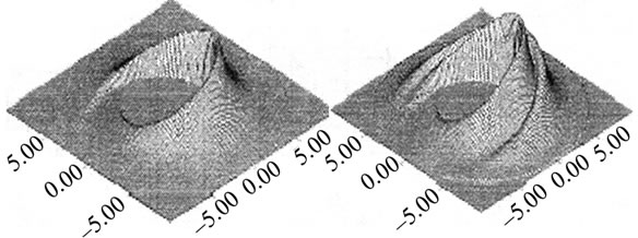 (b)
(b) (c)
(c)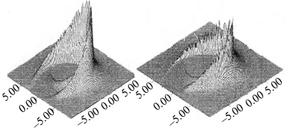 (d)
(d)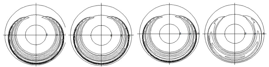 (d)
(d)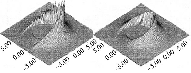 (a)
(a)
Figure 5. Contour lines of the intensity of the precipitating electron flux density for the nonstationary boundary conditions (results of the modeling).


Figure 6. Dynamics of aurora from the Polar satellite on January 6, 1998 at 1621-1717 UT [16].
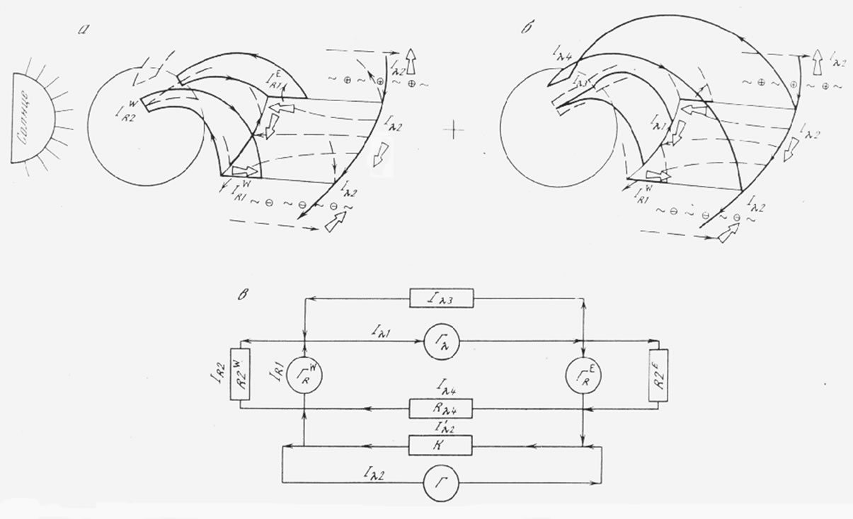
Figure 7. Schematic spatial location of the magnetospheric--ionospheric currents[7,8]: (a) the system of feeding the meridional currents, (b) the system of feeding the latitudinal currents, and (c) the equivalent scheme of the magnetospheric— ionospheric current circuit. The currents are shown by thin solid lines; electric fields, by open arrows; and convection, by dashed lines. The wavy line corresponds to the region of bulk charge localization. (G) electric energy generators, (C) MHD compressor, (R) ionospheric sections of the circuit with active load, and (I) corresponding currents.
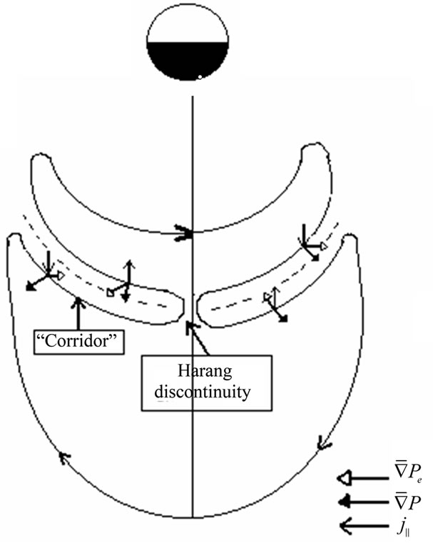
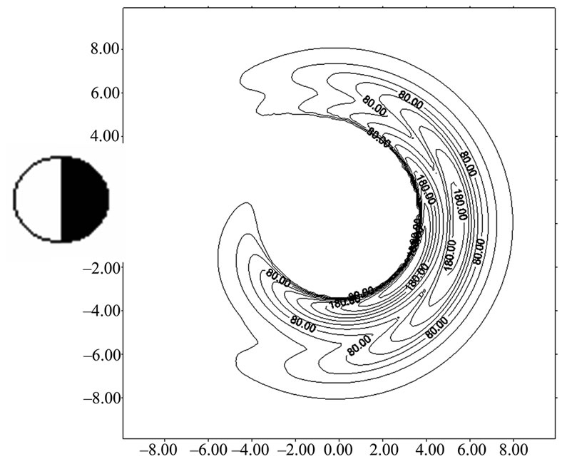
Figure 8. Schematic of the section of the gas pressure relief. The section of the “gorge” is represented by “corridors” or channels of magnetospheric MHD-generators, on the walls of which field-aligned currents are generated. The walls of the “corridors” serve as the sources of two bands of field-aligned currents, the direction of which is opposite on different walls. There arises a current configuration corresponding to the well-known Iijima and Potemra scheme. The prototypes of the channels—plasma “corridors” are located close to gas pressure maximum, i.e. maximum of particles precipitations into the ionosphere, where auroral electrojets are located [11].
Mi is the ion mass, ωiB is the ion gyrofrequency, and νin- the ion-neutral collision frequency.
On the other hand, the gas pressure gradient is responsible for the bulk density of the current: j ┴ = c[B ´ Ñpg]/B2, and the field-aligned currents are determined by divergence of the bulk currents, it is clear that the plasma pressure distribution is completely responsible for the field-aligned current pattern (Figure 9—the middle pan-
 (a)
(a)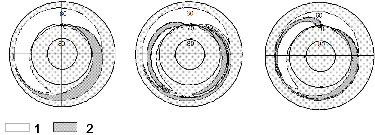 (b)
(b)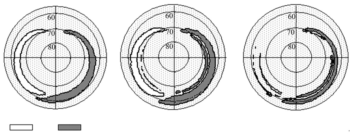 (c)
(c)
Figure 9. Results of calculations of the field-aligned currents ((a) t = 0 s, (b) t = 1000 s, and (c) t = 2800 s) generated in the ionosphere (the upper panels) and magnetosphere (the middle panels), as well as the comparison (compatibility) of these currents (the lower panels); (1) and (2) the zones of inflowing and outflowing currents, respectively.
els) and, consequently, for the scheme of feeding of the ionospheric current systems. The expression for thefield-aligned current [7,12,13]:
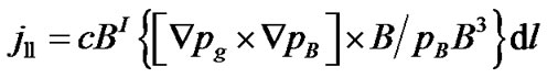
where ВI is the magnetic field strength in the ionosphere, the integral is taken over the entire flux tube from the equator to the ionosphere, and рВ is the magnetic pressure. It is clear that the integrand is proportional to the sine of the angle between the contour lines pg = const and pB = const.
Figure 9 shows the distribution of the field-aligned currents from the ionosphere (the upper panels) and magnetosphere (the middle panels) and the combined distributions (the lower panels) in the projection on the northern polar region. It is evident that the general construction of the field-aligned currents corresponds to the known empirical pattern [14].
The combination was performed in the following way. If the field-aligned current amplitude in a given zone was lower (higher) than the threshold density dependent on the noise level, index 0 (1) was attached to this amplitude. Both field-aligned current patterns were numbered in such a way and were subsequently multiplied. If the area occupied by unities in the ionospheric, magnetospheric, and combined patterns are denoted by Si, Sm, and Sc, the combination quality criterion will be the number:

K is mostly about 2% and only sometimes reaches 5%.
4. Discussion of Results and Conclusions
The problem of compatibility of field-aligned currents generated in the magnetosphere, and of field-aligned currents, which are produced as a result of a spatial inhomogeneity of conductivity (and to a lesser extent, of the electric field), that is, as if they were “generated” in the ionosphere, is part of the problem of ionospheremagnetosphere coupling. It is clear that in actual fact they are simply parts of one and the same global ionospheric-magnetospheric current system. The problem of ionosphere-magnetosphere coupling primarily implies that it is necessary to solve the question as to how the magnetospheric producer of current and power “adjusts itself” to the ionospheric consumer. For a certain special configuration, this problem was solved in [11,15].
It turned out, firstly, that the ionospheric consumer updates the convection rate and through it the plasma pressure gradient, which determines the density of bulk currents which, in turn, determines the behavior of fieldaligned currents through its divergence. Secondly, it turned out that ionospheric and magnetospheric currents are not rigidly linked. Some of the current (and power!) that is not “demanded” by the ionosphere can go into feeding the magnetospheric MHD compressor pumping plasma into the region of increase magnetic pressure - in the earthward direction [11].
The most important issue in this paper is that of ascertaining the direction of the cause-and-effect relationship. Electric current is primary in the magnetosphere, whereas the electric field is primary in the ionosphere. Furthermore, the convection system can undergo some adjustment, and together with it the electric field in the ionosphere. But such adjustment is possibly only as corrections of the first approximation to the zero-order approximation. And hence the zero-order approximation, that is, the picture of field-aligned currents obtained essentially for an arbitrary but smooth initial electric field must contain the main elements of the natural system of field-aligned currents which is determine by the distribution of electron precipitation closely associated with the plasma pressure distribution in the magnetosphere. Let us now consider from this standpoint Figure 9.
Figure 9 (the upper panels) shows a classical picture of field-aligned currents that coincides in its main traits with the well-known Iijima-Potemra scheme [14]. This correspondence indicates that the factor that determines the main features of the configuration of field-aligned currents is the existence in the ionosphere of a well conducting channel produced by zones of intense precipitation of electrons from the plasma pressure hump region (see Figures 1 and 3).
However, whether or not the enhancement of current in this channel with enhanced conductivity is possible will depend on whether the magnetospheric source is able to supply field-aligned currents this peculiar “discharge gap”, as shown in Figure 10.
Figure 9 shows the picture of field-aligned currents that is “offered” by the magnetosphere. One can see that “demand” and “supply” are more or less identical for the arrangements of the zones. It should be noted that the integral over all inflow and outflow currents in Figure 9 is virtually zero. Thus, we can state that the field-aligned currents, which resulted from the divergence of the ionospheric surface currents only due to nonuniformity of the ionospheric conductivity, and the magnetospheric currents, which resulted from the convergence of the contour lines of the gas and magnetic pressures, proved to be in rather good natural agreement.
In the paper [16] authors have executed comparison of such modeling calculations [7,8] with the data of satellite measurements for event on January, 6, 1998 (1621-1717 UT). For example, see Figures 5 and 6.
Unfortunately, direct observations of plasma distribution in the magnetosphere are faced with large difficulties, because pressure must be known everywhere in the
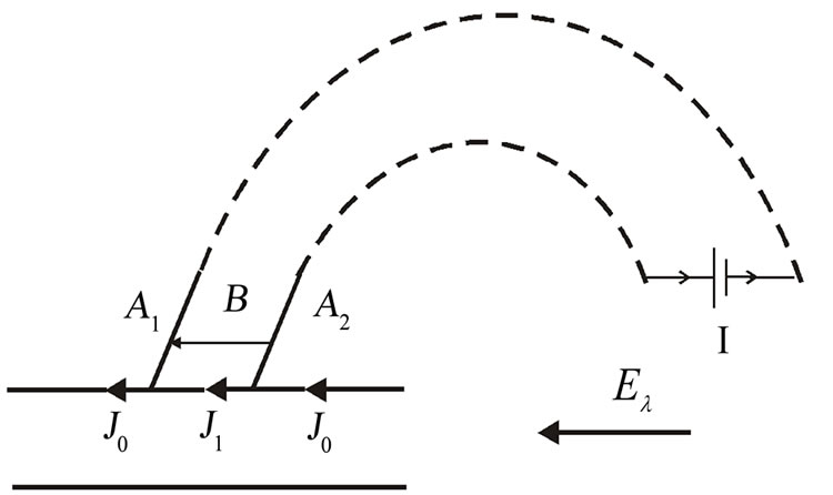
Figure 10. A—ionospheric region with background (low) conductivity. B—ionospheric region with increased electric conductivity. The portion A1-A2 has a large-scale (quasihomogeneous) meridional electric field EAl that produces the electric current. If the source of current I in the corresponding magnetospheric region is absent, then the current j flows in the entire portion A1-A2; however, the electric field in region B, EBl, is decreased. If, however, the source of current I is present in the magnetosphere, then El is everywhere identical, and on portion B the electric current jB is enhanced. Hence, in the former case jB = j0 and EBl < EAl, and in the latter case EBl = EAl, but jB = j0.
plasma sheet at high resolution, which in situ satellites have been unable to provide. As shown by Waters et al. [17], a map of global field-aligned currents can be constructed with hourly resolution using magnetometer data from the Iridium System consisting of 66 satellites in circular polar orbits. Modeling of distribution of plasma pressure (on ~3 - 10 Re) is very important, because the data from 66 satellites would be a very expensive mission. Although, multisatellite projects are very useful.
Perhaps, an enigma of a substorm may be in distribution of plasma pressure, or more exactly, in a global redistribution of plasma pressure on the night side of the magnetosphere. Although in previous papers by Harell, Wolf [18] there were essential lacks (see criticism of these papers in [7], but nevertheless, works in this direction now go on (see, for example, [19,20]).
9. References
[1] E. E. Antonova, N. Yu Ganushkina, “Azimuthal Hot Plasma Pressure Gradients and Dawn-Dusk Electric Field Formation,” Journal of Atmospheric and SolarTerrestrial Physics, Vol. 59, No. 11, 1997, pp. 1343-1354. doi:10.1016/S1364-6826(96)00169-1
[2] E. E. Antonova, “Radial Gradients of Plasma Pressure in the Magnetosphere of the Earth and the Value of Dst Variation,” Geomagnetism and Aeronomy, Vol. 41, No. 2, 2001, pp. 148-156.
[3] P. De Michelis, I. A. Daglis and G. Consolini, “An Average Image of Proton Plasma Pressure and of Current Systems in the Equatorial Plane Derived from AMPTE/ CCE-CHEM Measurements,” Journal of Geophysical Research, Vol. 104, No. 12, 1999, pp. 28615- 28624.
[4] A. S. Kovtukh, “Radial Profile of the Pressure of the Storm Ring Current as a Function of Dst,” Cosmical Research, Vol. 48, No. 3, 2010, pp. 218-238, (in Russian).
[5] M. V. Stepanova, E. E. Antonova, J. M. Bosqued and R. Kovrazhkin, “Azimuthal Plasma Pressure Reconstructed By Using the 3 Aureol-3 Satellite Data During Quiet Geomagnetic Conditions,” Advances in Space Research, Vol. 33, No. 5, 2004, pp. 737-741.
[6] C. F. Kennel, “Consequence of a Magnetospheric Plasma,” Review of Geophysics, Vol. 7, No. 1-2, 1969, pp. 379-419. doi:10.1029/RG007i001p00379
[7] E. A. Ponomarev, “Mechanism of Magnetospheric Substorms,” Nauka, Moscow, 1985, p. 157, (in Russian).
[8] E. A. Ponomarev and P. A. Sedykh, “How Can We Solve the Problem of Substorms? Geomagnetism and Aeronomy,” Pleiades Publishing, Vol. 46, No. 4, 2006, pp. 560-575.
[9] K. Birkeland, “The Norvegian Auгora Polaris Expedition 1903-1908,” Christiania, Vol. 1, 1913, pp. 1220-1224.
[10] R. A. Bostrom, “A Model of the Auroral Electrojets,” Journal of Geophysics Research, Vol. 69, No. 23, 1964, pp. 4983-4987. doi:10.1029/JZ069i023p04983
[11] P. A. Sedykh and E. A. Ponomarev, “The Magnetosphere-Ionosphere Coupling in the Region of Auroral Electrojets,” Geomagnetism and Aeronomy, Pleiades Publishing Inc., Vol. 42, No. 5, 2002, pp. 613-618.
[12] V. M. Vasyliunas, “Mathematical Models of Magnetospheric Convection and its Coupling to the Ionosphere,” In: B. M. McCormac Ed., Particles and Fields in the Magnetosphere, Higham, 1970, pp. 60-71.
[13] B. A. Tverskoy, “Electric Fields in the Magnetosphere and the Origin of Trapped Radiation,” Solar-Terrestrial Physics, Dordrecht, 1972, pp. 297-317.
[14] T. Iijima and T. A. Potemra, “Large-Scale Characteristics of Field-Aligned Currents Associated with Substorms,” Journal of Geophysics Research, Vol. 83, No. A2, 1978, pp. 599-615. doi:10.1029/JA083iA02p00599
[15] E. A. Ponomarev, P. A. Sedykh and V. D. Urbanovich, “Bow Shock as a Power Source for Magnetospheric Processes,” Journal of Atmospheric and Solar-Terrestrial Physics, Vol. 68, No. 6, 2006, pp. 685-690. doi:10.1016/j.jastp.2005.11.007
[16] S. I. Solovyev, “Magnetosphere-Ionosphere Response to Magnetosphere Compression by the Solar Wind,” Proceeding of XXVI Annual Seminar, Apatity, 2003, pp. 41-44.
[17] C. L. Waters, B. J. Anderson and K. Liou, “Estimation of global Field-Aligned Currents Using the Iridium System Magnetometer Data,” Geophysical Research Letters, Vol. 28, No. 11, 2001, pp. 2165-2168. doi:10.1029/2000GL012725
[18] M. Harell, R. A. Wolf and P. H. Reif, “Quantitative Simulation of a Magnetospheric Substorm, 1. Model Logic and Overview,” Journal of Geophysical Research, Vol. 86, No. A4, 1981, p. 2217. doi:10.1029/JA086iA04p02217
[19] R. A. Wolf, Y. Wan, X. Xing and J. C. Zhang, “Sazykin S. Entropy and Plasma Sheet Transport,” Journal of Geophysical Research, Vol. 114, 2009. doi:10.1029/2009JA014044
[20] L. R. Lyons, C. Wang, M. Gkioulidou and S. Zou, “Connections between Plasma Sheet Transport, Region 2 Currents, and Entropy Changes Associated with Convection, Steady Magnetospheric Convection Periods, and Substorms,” Journal of Geophysical Research, Vol. 114, 2009, p. 14. doi:10.1029/2008JA013743