Journal of Sensor Technology
Vol. 2 No. 2 (2012) , Article ID: 19674 , 5 pages DOI:10.4236/jst.2012.22008
Acousto-Optic Measurement Device with High Angular Resolution
V. E. Zuev Institute of Atmospheric Optics Russian Academy of Sciences, Siberian Branch, Tomsk, Russia
Email: *gkaloshin@iao.ru
Received August 26, 2011; revised October 28, 2011; accepted November 20, 2011
Keywords: Laser Beam; Acousto-Optical Device; Diffraction; Atmospheric Turbulence
ABSTRACT
The paper introduces a new laser interferometry-based method for diagnosis of random media by means of high accuracy angle measurements and describes the results of its development and testing. Theoretical calculations of the dependence of the range of the laser interferometer on laser beam parameters, device geometry, and atmospheric turbulence characteristics are reported. It is demonstrated that at moderate turbulence intensities corresponding to those observed most frequently in turbulent atmosphere at moderate latitudes and with low interference contrast values, the performance range of the laser interferometer-based device exceeds 5 km.
1. Introduction
State-of-the-art level of development of acousto-optic devices allows for their wide application, particularly in diagnosis of random media by means of high accuracy angle measurements [1-3]. These may be applied in the control of transient processes in gaseous and liquid media, plasma, turbulent atmosphere, and also in geodesy, ranging, and navigational course detection. Modern photo acoustic grating deflectors (PAD) are characterized by high resolution and fast response. Along with the simple design, ease of control, low power consumption, and small size, these advantages arouse interest in using PADs for atmospheric laser interferometers. A fundamental problem here lies in ensuring high precision in the measurement of angles, which may be, at least, 5000 times smaller than 1 second of arc.
References [4,5] introduce a method, in which during synchronous scanning of two laser beams in the region of their superposition, wave interference is observed, and frequency of the resultant oscillation is uniquely associated with the source direction. It is known that the possibility of registering interference contrast is determined by the presence of random nonuniformities in permittivity of air on the path. Therefore, it appears interesting to estimate an operation range of the method, depending on turbulence characteristics and optical scheme parameters of the device.
2. Interferometric Method of Specifying Direction
An optical schematic of the atmosphere laser path interferometer (Laser Interferometer—LI) employing this method for a one-dimensional case is shown in Figure 1. (For a two-dimensional case, a laser beam is scanned across two coordinates using either two one-dimensional PADs in tandem or one PAD cell, in which two orthogonal acoustic waves are excited).
A laser beam passes sequentially through two acoustic cells, PAD-1 and PAD-2, whose medium density is varied under the influence of ultrasound from a sweep-frequency generator. The acoustic waves produce a phase grating on which laser radiation is diffracted. With the help of collimators of a beam forming device, further referred to as BFD, and diffracted beams are directed towards the atmosphere path, where they produce an interference pattern in the region of mixing. Characteristics of the optical system and positioning of the optical elements are chosen so that polarization of both beams and their intensities are similar.
A photo detector registers and separates the received signal frequency, which uniquely correlates with direction to BFD.
Position of the laser beams in space is determined by the relation , where
  is the diffraction (scanning) angle;
  is the optical radiation wavelength in vacuum;
  is the acoustic wave frequency; na is the acoustic wave speed in a PAD. At small diffraction angles, this may be transformed to
 . For a He-Ne laser (l = 0.63 mm) and acoustic wave frequency fa = 10 × 106 Hz,
 . If
. If  is increased 10-fold by means of optical amplification, the diffraction angle of 1 second of arc corresponds to the frequency of 5.5 kHz.
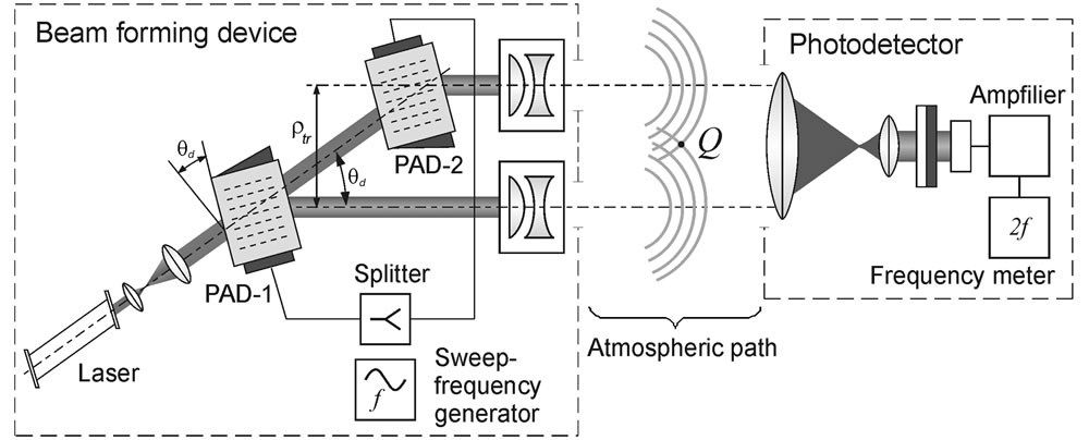
Figure 1. The schematic of the atmospheric laser path interferometer.
Hence, setting direction to within 1 second of arc is not technically challenging. As such, the accuracy of measurements may exceed at least 1/5000 seconds of arc. This unveils wide opportunities in application of the method both in research and engineering. In particular, it may be valuable in optical refraction spectroscopy, photothermal deflection spectroscopy for the control of transient processes in gaseous and liquid media and plasma, in atmospheric optics for the study of intensity fluctuations during the propagation of optical radiation, in investigation of mirage detection and reflectance techniques, in geodesy, optical profilometry, ranging, and navigational course detection. It may be valuable for control not steady-flow process where now used laser remote techniques. Thus possibilities of these methods it is limited by the sizes of laser beams. LI method has essentially best possibilities by the resolution as in it the resolution is defined by width of an interference band.
3. Distortions of an Interference Pattern Formed by a PAD
Various aspects of interference pattern formation in turbulent atmosphere have been studied in References [6-8]. For the purpose of this paper, we summarize a theoretical approach described in References [7,8] applying it to a more realistic model of optical radiation sources.
Let us consider the following model of a BFD and a photodetector: coherent radiation sources located at the points  and
and , respectively, emit laser beams parallel to each other and the OX-axis in the direction of positive x growth; the photodetector is located at point Q (see Figure 1) with coordinates
 . Vector
  denotes spacing between the radiation sources producing the interference pattern.
Let optical radiation from each source be represented as a partially coherent Gaussian beam with initial amplitude U0, initial radius a0, radius of the wave front curvature in the center of radiating aperture R0, and initial coherence radius rk. An assumption about complete identity of the sources somewhat simplifies the problem without introducing serious restrictions. The photodetector is represented as a quadratic detector, which reacts to intensity of arriving radiation, and its signal is proportional to instantaneous interference pattern intensity at the detector location, which can be written as
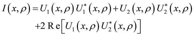 (1)
(1)
where  is the optical wave field of one source; j = 1, 2. In the following we consider that
  and
and .
.
For the above-formulated boundary conditions, an equation describing the function of mutual second-order field coherence for two Gaussian optical radiation beams has the following solution when using quadratic approximation of the structural function of fluctuations of a complex optical wave phase:
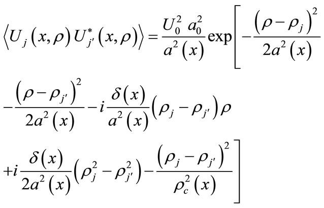 (2)
(2)
where
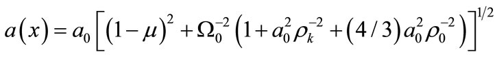
is the mean radius of the optical radiation beam;
is a geometrical factor related to mutual curvature of the mean wave fronts of the beams;
is the radius of mutual coherence of the two optical beams; m = x / R0 is the focusing parameter;  is the Fresnel number of the radiating aperture; k = 2p/l is the optical wave number;
  is a coherence radius of a plane optical wave in turbulent atmosphere;
  is a structural fluctuations parameter of dielectric permittivity in turbulent atmosphere; j, j¢ = 1, 2. Using Equations (1) and (2), it is possible to obtain an expression for mean intensity of the interference pattern produced by two partially coherent laser beams in turbulent atmosphere. The latter allows specifying simple and intuitive conditions for restricting the choices of laser beam parameters and BFD schemes using standard characteristic values for atmospheric turbulence above the sea surface [7,8].
If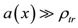 , linear dimensions lint(x) of the region of formation of the interference pattern are described using a value approximately equaling the laser beam diameter:
 (3)
(3)
The interference band maxima are located at points pmax, while the minima are located at points pmin. For simplicity, let us assume that . Then, interference band width Dlint(x) can be assessed using equation
 (4)
(4)
At the same time, visibility of a distorted interference pattern obtained using average intensity when pmax ≈ pmin ≈ p, is equal to
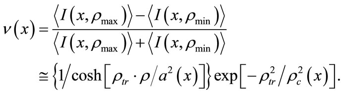 (5)
(5)
It is evident that the method works only if there is at least one complete interference band in the interference image field; therefore, the following necessary condition follows from Equations (3) and (4)
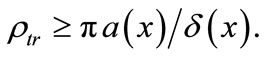 (6)
(6)
Additionally, visibility of the middle interference pattern is satisfactory as long as the coherence radius of the registered optical field exceeds the magnitude of transverse displacement of the beams at the point of observation. Hence, when considering visibility near the centre of the interference pattern, by simplifying Equation (5) one obtains
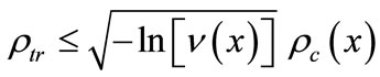 . (7)
. (7)
By combining Equations (6) and (7), the following equation is derived:
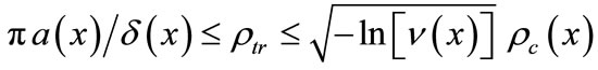 (8)
(8)
In order to fulfill Equation (8), the right part must at least exceed the left part; otherwise (in the case of collimated beams m = 0) this is equivalent to a requirement to limit the initial size of the laser beams a0 to obey the condition:
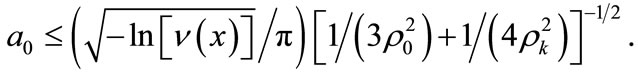 (9)
(9)
It must be noted that for horizontal atmospheric paths not longer than 10 km, Equation (9) imposes quite severe limitations on the laser beam parameters, which may only be satisfied for sufficiently narrow and highly coherent laser beams.
4. Choice of Parameters for the LI Optical Scheme
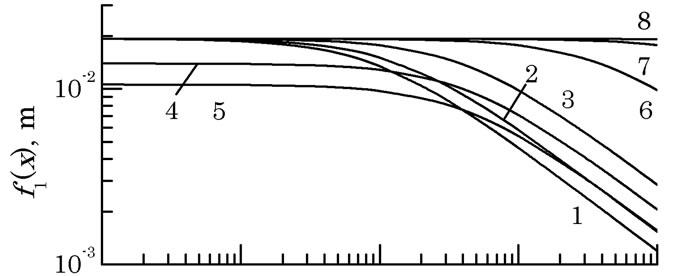
Figure 2(a) shows plots of the function
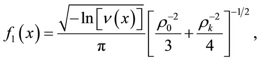
for different values of parameters of the problem. Curves 1, 2, and 3 demonstrate the influence of optical radiation wavelength l on function f1(x): 1 – l = 0.51, 2 – 0.63, and 3 – 1.06 mm (other parameters are as follows: rk = 2 cm, v(x) = 0.1,  = 10–13 m–2/3); curves 3, 4, and 5 demonstrate sensitivity of f1(x) to the contrast of the interference pattern v(x): 3 – v(x) = 0.1, 4 – 0.3, 5 – 0.5 (in this case, l = 1.06 mm, rk = 2 cm,
  = 10–13 m–2/3), while curves 3, 6, 7, and 8 show the dependence of f1(x) on the level of dielectric permittivity fluctuations in turbulent atmosphere
 : 3 –
: 3 – = 10–13 m–2/3, 6 – 10–14, 7 – 10–15, 8 – 10–16 m–2/3 (l = 1.06 mm, rk = 2 cm, v(x) = 0.1). It appears that in order for condition (9) to be satisfied with the path length range 1 m to 10 km, initial radii of the laser beams a0 must not exceed 1 - 2 mm.
At known parameters of the optical beams, Equation (8) allows choosing the distance rtr between the radiation sources, producing the interference pattern. Figure 2(b) demonstrates plots of the functions
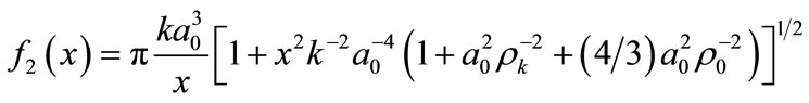
(solid lines) and
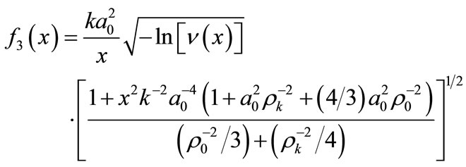
(dashed lines) calculated for different values of the parameters of the problem.
 (a)
(a)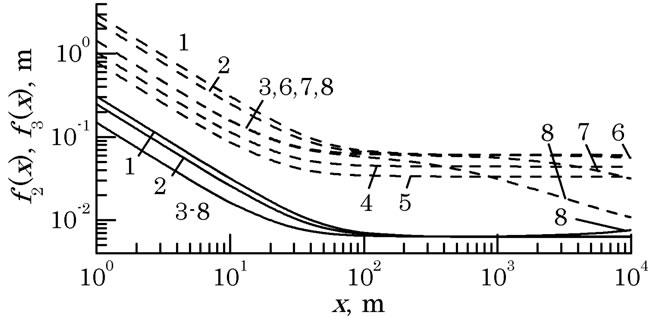 (b)
(b)
Figure 2. Nomograms used for the selection of initial values of laser beam parameters and spacing of their optical axes.
Curves 1, 2, and 3 indicate the influence of l on f2(x) and f3(x): 1 – l = 0.51, 2 – 0.63, and 3 – 1.06 mm (in this case, a0 = 2 mm, rk = 2 cm, v(x) = 0.1,  = 10–16 m–2/3), curves 3, 4, and 5 are calculated, respectively, for the following values of the interference contrast v(x): 0.1 (3), 0.3 (4), and 0.5 (5) (other parameters are constant: l = 1.06 mm, a0 = 2 mm, rk = 2 cm,
  = 10–16 m–2/3), while curves 3, 6, 7, and 8 are calculated for different levels of dielectric permittivity fluctuations of turbulent atmosphere
 : 10–16 m–2/3 (3), 10–15 m–2/3 (6), 10–14 m–2/3 (7), and 10–13 m–2/3 (8) (l = 1.06 mm, a0 = 2 mm, rk = 2 cm, v(x) = 0.1). Since the spacing rtr between the radiation sources producing the interference pattern, must exceed the value of f2(x) and be below the value of f3(x), it is possible to estimate acceptable values of rtr within the 1 - 5 cm range from Figure 2(b) for path lengths from 20 m to 10 km.
5. Assessment of the LI Ranging
As far as the major limitation for the range of action of a LI in turbulent atmosphere is related to decreasing visibility of the interference pattern, in accordance with Equation (7), the required estimate can be obtained by solving a nonlinear equation of the form
 (10)
(10)
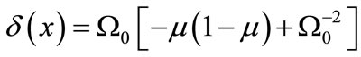
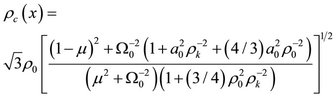
in which
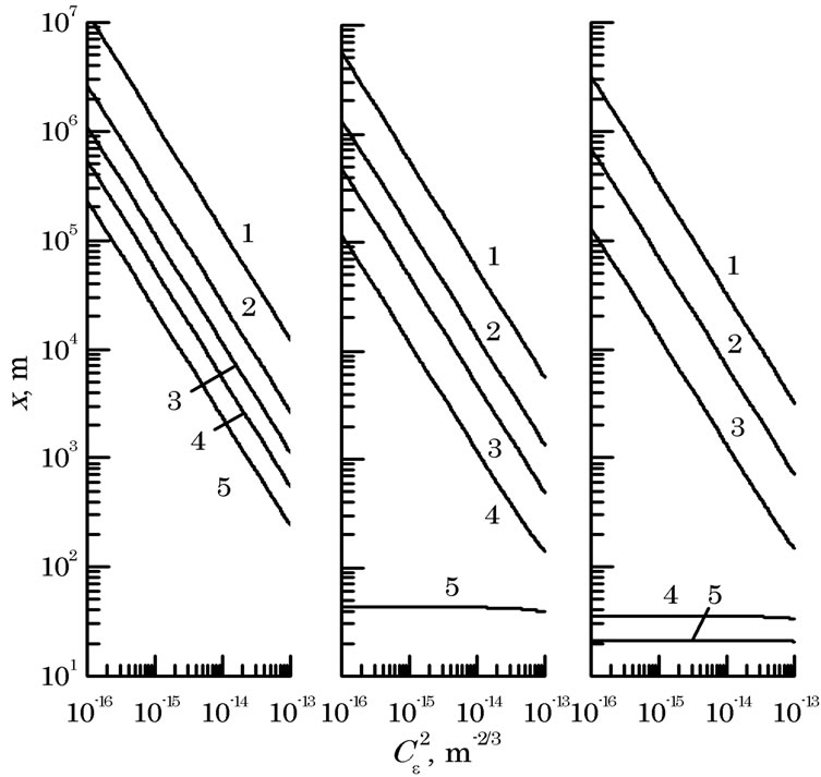
Equation (10) has been solved by the simple iterations method. Results of the estimates of the range of action of a LI are presented in Figure 3 for all values of the structural parameter of air permittivity fluctuations, valid for the near-water atmospheric layer [7,8], and for three values of interference pattern visibility and optical radiation wavelength l = 1.06 mm. It is assumed that the laser radiation propagated along a horizontal path at the height of 10 - 20 m above the water surface.
6. Conclusions
Based on the results presented in this work, the following conclusions can be drawn:
1) A decrease in the distance between the optical radiation sources results in lowering of the contrast value of the registered interference pattern; while an increase in the radiation wavelength results in a growth in the range of BFD;
2) At a lower value of the optical wavelengths interference pattern contrast (v(x) = 0.1), the device ranging exceeds 5 km , for the source spacing of 1 to 5 cm, and the mean turbulence intensity of 10–15 m–2/3 which is most commonly observed in the turbulent atmosphere at moderate latitudes;
3) At higher interference pattern contrast values, in order for the laser interferometer to operate efficiently the spacing rtr of radiation sources producing the interference pattern reduces (ranging from 1 to 4 cm for v(x)
 (a) (b) (c)
Figure 3. Laser beam range as a function of the structural parameter of atmospheric turbulence at radiation wavelength l = 1.06 mm and interference pattern visibility v(х) = 0.1 (a), 0.3 (b) and 0.5 (c) for different distances between the beam centers rtr = 0.01 (1), 0.02 (2), 0.03 (3), 0.04 (4), and 0.05 m (5).
= 0.3, and from 1 to 3 cm at v(x) = 0.5).
In summary, this paper describes the operation of an atmospheric laser path interferometer based on the mean intensity analysis of a PAD-formed interference pattern used for specifying interference of BFD parameters, thereby providing the required range of operation for the LI above the ground surface for all possible values of turbulence parameters in weakly turbid atmosphere.
REFERENCES
- N. Savage, “Acousto-Optic Devices,” Nature Photonics, Vol. 4, 2010, pp. 728-729. doi:10.1038/nphoton.2010.229
- V. I. Balakshy and D. E. Kostyuk, “Application of Bragg Acousto-Optic Interaction for Optical Wavefront Visualizetion,” Proceedings of the International Society for Optics and Photonics, Vol. 5953, 2005, pp. 136-147.
- V. B. Voloshinov, T. M. Babkina and V. Y. Molchanov, “Two-Dimensional Selection of Optical Spatial Frequencies by Acousto-Optic Methods,” Optical Engineering, Vol. 41, No. 6, 2002, pp. 1273-1280. doi:10.1117/1.1477437
- G. A. Kaloshin and V. M. Shandarov, “The Device for Moving Objects Orientation,” Inventor’s Certificate No. 1554605 SSSR, MKI4 G01s17/00, G01c21/04, 1988.
- G. A. Kaloshin and V. M. Shandarov, “The Method for Moving Objects Orientation,” Inventor’s Certificate No. 1804214 SSSR, MKI4 G01s17/00, 1988.
- E. Wolf, “Introduction to the Theory of Coherence and Polarization of Light,” Cambridge University Press, Cambridge, 2007.
- L. C. Andrews and R. L. Phillips, “Laser Beam Propagation through Random Media,” 2nd Edition, SPIE Press, Bellingham, 2005.
- V. E. Zuev, V. A. Banakh and V. V. Pokasov, “Optics of Turbulent Atmosphere,” Gidrometeoizdat, Leningrad, 1988.
NOTES
*Corresponding author.