Journal of Transportation Technologies
Vol.3 No.1(2013), Article ID:27016,16 pages DOI:10.4236/jtts.2013.31001
FPGA-Based Traffic Sign Recognition for Advanced Driver Assistance Systems
Department of Electrical and Computer Engineering, Illinois Institute of Technology, Chicago, USA
Email: erdal@ece.iit.edu
Received October 11, 2012; revised November 12, 2012; accepted November 26, 2012
Keywords: Traffic Sign Recognition; Advanced Driver Assistance Systems; Field Programmable Gate Array (FPGA)
ABSTRACT
This paper presents the implementation of an embedded automotive system that detects and recognizes traffic signs within a video stream. In addition, it discusses the recent advances in driver assistance technologies and highlights the safety motivations for smart in-car embedded systems. An algorithm is presented that processes RGB image data, extracts relevant pixels, filters the image, labels prospective traffic signs and evaluates them against template traffic sign images. A reconfigurable hardware system is described which uses the Virtex-5 Xilinx FPGA and hardware/software co-design tools in order to create an embedded processor and the necessary hardware IP peripherals. The implementation is shown to have robust performance results, both in terms of timing and accuracy.
1. Introduction
Advances in materials, engine design, embedded electronics, and production methods have made the personal vehicle one of the most transformative technologies of the past century [1,2]. With cars becoming almost ubiquitous in developed nations, there has also been a large rise in associated risks. According to the US Census Bureau in 2009 alone 10.8 million motor vehicle accidents occurred resulting in almost 36 thousand fatalities. As horrible as these number are, they are a significant improvement from the previous decade. In 1990 there were 11.5 million accidents resulting in 46.8 thousand deaths [3]. This marked reduction in accidents (6%) and fatalities (23%) despite the population increasing by nearly 10% [4] is a testament to the efforts being made to driver safety and accident avoidance. Technologies like airbags, antilock brakes, tire pressure monitors, and traction control have become very common if not standard. More recently a new level of intelligence and intervention has surfaced in the form of systems commonly referred to as Advanced Driver Assistance Systems (ADAS) such as lane departure warning systems, intelligent speed adaptation, and driver drowsiness detection [5]. These technologies have the capacity to greatly increase driver safety by monitoring the driver and their environment and providing information, warnings, or even taking action. Traffic sign recognition (TSR) is one of these technologies.
Over the years, as our road system has matured, road signs have become the de facto way of communicating information to the driver. These road signs communicate the local traffic laws, such as right of way and speed limits as well as information like city limits and distances to destinations. Road signs, however, are only useful if the driver notices them. Though this fact is inherently obvious, it nonetheless is worth noting because it highlights the fact that increasing a driver’s ability to see road signs can increase road safety [6]. A driver may be distracted, tired, or simply overwhelmed driving in a new environment and miss an important road sign. A system that monitors the road ahead of a vehicle and detects road signs could be a great service to the driver. This information, summarizing the traffic sign topology of the area, could be displayed to the driver or used in conjunction with other vehicle information to take action such as slowing the vehicle as it approaches a stop sign.
This paper describes in detail a specific implementation of a traffic sign recognition system done in reconfigurable hardware. Following section discusses the challenges encountered for building traffic sign recognition systems and briefly describes existing research and product embodiments in this technology. The subsequent sections detail the algorithm design, the actual hardware implementation, and performance results.
A traffic sign recognition system monitors a complex and ever changing environment and must do so accurately and continuously. Here in lies the challenges for this type of system: complex environment, expectation of accuracy, and short response time. Essentially it must identify the road signs that are in view in real time. These efforts to determine the presence of a road sign in real time are complicated by the fact that the environment is continually changing. Road signs will appear significantly different to an artificial (i.e., computer) vision system depending on the amount, direction, and type of light as well as weather conditions. Road signs may also be damaged or tilted confusing an automated system.
2. Background
Traffic sign recognition is an arena of active research. Although there are many different algorithms and approaches, some patterns do emerge as the existing body of work is examined. The following is a summary of some of the more recent and relevant work.
Lai et al. [7] present a sign recognition scheme aimed for intelligent vehicles and smart phones. Color detection is used and is performed in HSV color space. Template based shape recognition is done by using a similarity calculation. OCR is used on the pixels within the shape boarder to determine provide a match to actual sign. The description is purely algorithmic and implemented in software. Andrey et al. [8] use a very similar approach involving color segmentation and shape analysis. Histograms, however, are used as the shape classification method after connected regions are labeled. Actual sign recognition is done via template matching by using a weighted direct comparison of the interior portion of each shape to templates.
A different approach is used by Soendoro et al. [9]. Here, a binary image is created using color segmentation. Morphological filtering is used to improve the image. Shape estimation is done by an application of Ramer-DouglasPeucker algorithm followed by classification using Support Vector Machines (SVM).
Liu et al. [10] limit their application to speed limit signs found in Europe, Asian, and Australia. This causes their target signs to all be outlined in a red circle. The Canny edge detection algorithm is applied followed by the Fast Radial Symmetry Transform to detect circular signs. A fuzzy template matching, a comparison of correlation coefficient is used to initially match the information within the circular sign. A character recognizer based on the local feature vector is used to make the final match selection. This algorithm is implemented in software running on a standard PC.
A novel approach is described by Kastner et al. [11]. They use the difference of Gaussian and Gabor filter kernels to model the characteristics of neural receptive fields measured in the mammal brain. They attempt to process an image in a similar way that human’s brains do. This highlights areas of important information in a frame identifying regions of interest (ROIs). These ROIs have relevant information extracted in the form of week classifiers, essentially a probability value that corresponds to a certain traffic sign class. Their algorithm is implemented on a standard PC running software.
The bulk of the research materials on this topic have focused on algorithms that are implemented in software. A few have been targeted toward reconfigurable hardware, but even these often have all or a large portion of the work performed by an embedded processor running software. Souki et al. [12] describe an algorithm implemented on FPGA-Cyclone II 2C35 FPGA manufactured by Altera. They use color segmentation to create a binary image. Edge detection and Hugh Transforms are use to detect shapes. Classification uses template matching. This algorithm is implemented exclusively in software that runs on the Nios II embedded processor. Computation times exceed 17 seconds per frame.
Designed using SystemC, Muller et al. [13] present a system that uses a Virtex-4 LX100 FPGA with implementations of multiple embedded LEON CPU cores. Their algorithm of preprocessing, shape detection, segmentation, extraction, and classification, is initially implemented exclusively in software. To improve their performance they move the classification stage to a synthesized hardware block. With this improvement they are able to achieve a computation time of about 0.5 seconds.
Similarly, Irmak [14] uses an embedded processor approach with minimal support from portions of the algorithm implemented in hardware. Color segmentation, shape extraction, morphological operations and template matching are all performed in the Power PC processor that is part of the system. Only edge detection is implemented in hardware.
In addition to being a topic of active academic research, Traffic Sign Recognition is also a technology that is being researched and implemented in the industry. This technology is developed by many car manufacturers who are partnering with traditional automotive suppliers such as Continental Automotive, TRW, Bosch [15] and newer image recognition software product developers like Ayonix. Continental Automotive developed several products for traffic sign recognition. Its Multi Function Camera specification details its abilities for use in TSR [16]. This traffic sign recognition system [17] began production in 2010 on the BMW 5-series. In addition to BMW, many other carmakers have rolled out some version of this technology. Volkswagen has done so on Phaeton and the Audi A8. Mercedes-Benz E and S class both have an implementation of TSR. As well as the Saab 9-5, Opel, Insignia, and the European 2011 Ford Focus. Additionally, Google has developed technology that allows a vehicle to drive itself. Using a combination of data stored in its map database and data that it collects from its environment in real-time, the Google Car is able to safely navigate complex urban environments [18].
3. Algorithm Design
3.1. Algorithm Overview
The problem of identifying traffic signs within an image can be broken into the two sub-problems of detection and recognition. Detection presents the challenge of analyzing the image to identify portions of the image that could contain a traffic sign. Recognition is the challenge of determining if these candidates are indeed traffic signs and if so which one.
Figure 1 depicts the proposed algorithm used for detection and recognition of traffic signs. The following sections discuss each portion of the algorithm and present the specifics of the implementation of each part.
3.2. Hue Calculation and Detection
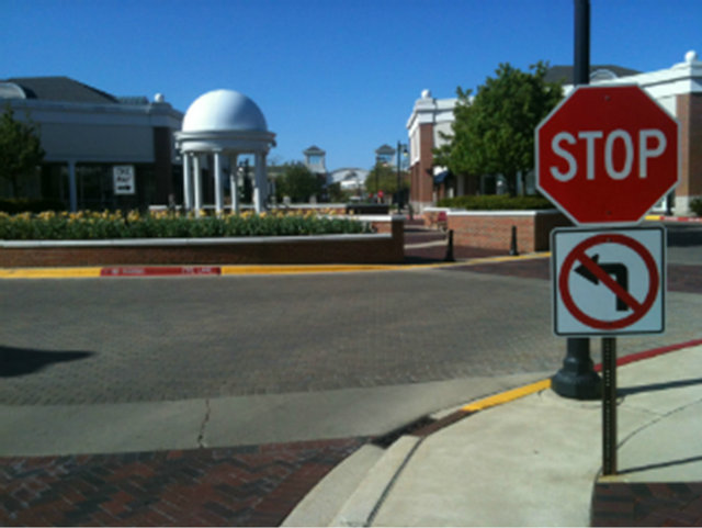
Traffic signs consist of solid color text, symbols, or shapes on a solid color background as seen in Figure 2. Scanning an image looking for this color signature will allow for the quick identification of possible traffic signs and the rejection of the remaining parts of the image.
Stop, yield, do not enter, wrong way, and prohibition signs such as no left turn, all contain red backgrounds with white text or white backgrounds with red text. Main distinguishing color for these signs is red. Similar groupings can be done for signs that are primarily green, yellow, blue, or black and white. The algorithm described here and in the sections following must be performed for each of these color groupings.
For each group of similarly colored signs, the algorithm begins by scanning the image to calculate the hue of each pixel. There are a variety of ways in which to express the color of a pixel. Perhaps the most common is by using the color’s primary color components or the RGB value. Although this is very useful when displaying that color, it is not as helpful when trying to extract all the pixels of a specific hue. If, as in this case, the desire is to identify all the pixels that would be considered red, there are colors that contain a significant about of red as a primary color contributor, but are themselves not red. The color yellow is one such example. Figure 3(a) depicts the color representations using RGB.
To determine the hue of a pixel, or its color regardless of shade, a conversion must be made. Each RGB pixel is converted to a different triplet called HSV: Hue, Saturation, and Value. HSV represents the color spectrum by having a value for the color (hue), the amount of that color (saturation), and the brightness of that color (value) [19]. The hue parameter represents the angle where the pixel’s color lies on the cylinder depicted in Figure 3(b). Thresholds can be chosen to categorize any hue value found. Once this conversion is made, the hue values for each pixel can be scanned. Detection is the process of identifying the pixels whose hue value falls between the thresholds for the relevant color. This will split the image into two categories: pixels that have the hue of interest and those that do not. At this point the full color image being processed can be simplified into a binary image. Active pixels had the desired hue while inactive pixels do not. This step is called Hue Detection.
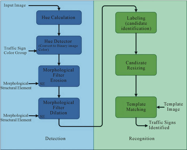
Figure 1. Algorithm flow chart.
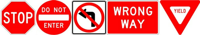
Figure 2. Example traffic signs (red).
 (a)
(a)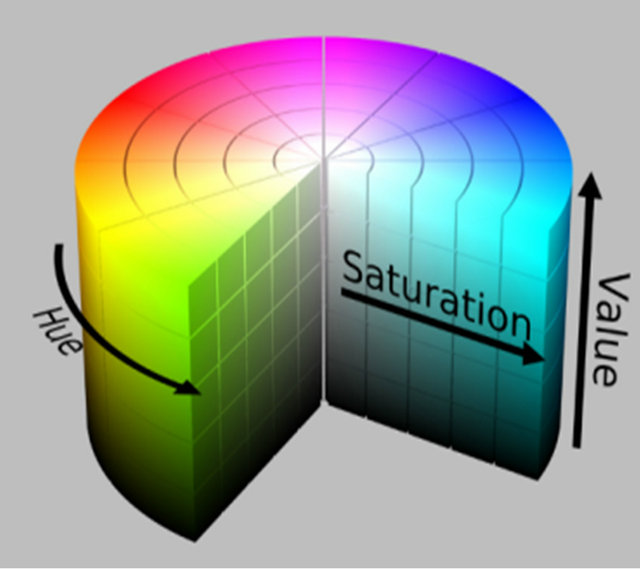 (b)
(b)
Figure 3. (a) RGB color space, (b) HSV color space [19].

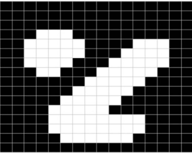
Figure 4. Hue calculation and detection example.
Figure 4 shows the effect of Hue Calculation and Detection on an example image. The red pixels have been extracted and are now represented in the binary image as active white pixels. Pixels of all other colors are represented as inactive or black pixels. At this point the system has eliminated a significant amount of information to consider it its effort to identify traffic signs. However, in many images a peppering of red pixel groupings will be found throughout. If each pixel grouping that remains were to be considered a potential traffic sign, most of these would clearly not be good candidates. A step is required where many of these small pixel groupings can be eliminated without adversely affecting the pixel groupings that are actually traffic signs. This measurement and others are deliberate, using specifications that anticipate your paper as one part of the entire journals, and not as an independent document. Please do not revise any of the current designations.
3.3. Morphological Filtering
Morphological transformation is a technique for processing digital images by exploiting the relationship between each pixel and its neighboring pixels. This relationship is defined by the type of morphological transformation and the structural element used. There are two basic transformations: Dilation and Erosion. These two can also be combined to create the Open and Close transformations. The structural element is essentially a small geometric shape such as a square, disk, line, or cross. During a transformation operation, each pixel is compared to its neighbors as defined by the window specified by the structural element. During erosion, the pixel in question will be deactivated unless all of the other pixels in the structural element window are also active. During dilation, the pixel will be activated if any of the other pixels in the structural element window are active. As their names might suggest, erosion has the effect of trimming the edges of objects where dilation has the effect of puffing out the edges [20,21]. Open and close operations are achieved by combining erosion and dilation. An open is obtained by erosion followed by dilation and a close is a dilation followed by erosion. The results of these operations are less dramatic because the second step tends to temper the effects of the first. Figure 5 shows example morphological transformations, erosion and dilation.
3.4. Labeling
After detecting the pixels in the image that match the desired hue and after filtering the resulting binary image to reduce the number of pixel “blobs”, the resulting image is ready for the labeling step. Labeling is the process of scanning the image to detect pixel groupings. Pixels that share an edge or a vertex are considered to be members of the same pixel grouping or “blob”. The remainder of this section will detail our proposed algorithm used to detect these blobs.
The goal with labeling is to identify a bounding box for each and every pixel grouping in the image. This will result in four parameters for every blob: Xmin, Ymin, Xmax, Ymax. These are the two diagonal corners that define the bounding box. Simply put, the labeling algorithm scans the image from bottom to top and left to right (raster order) keeping track of Xmin, Ymin, Xmax, Ymax for all the pixel groupings it encounters. During this scanning only one row plus 2 pixels are stored and labeled at a time. Labels are assigned and a table built containing the Xmin, Ymin, Xmax and Ymax values for each label. While scanning, a window of 5 pixels is examined at a time: the current pixel and its 4 previously visited neighbors. Each pixel initially starts with a label of 0 (not labeled) and if the pixel is a foreground pixel then a non-zero label is assigned. The value of that label
 (a)
(a)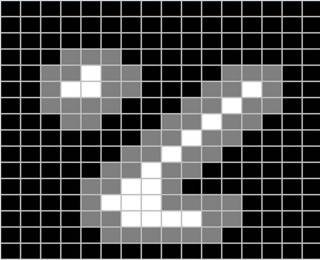 (b)
(b)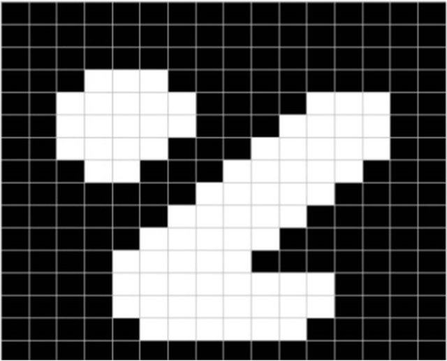 (c)
(c)
Figure 5. Morphological transformation example: (a) Original image; (b) After erosion operation with 3 × 3 square structural element (gray pixels are removed); (c) After dilation operation (yellow pixels added to the original).
depends on the labels of its four neighbors.
Figure 6 shows all the possible combinations for consideration when determining the label of the current pixel. Each of these diagrams represents the current pixel, X, its immediately previously scanned neighbor, P, and it’s previously scanned neighbors 1, 2, and 3. Shaded pixels are active and labeled. The key to this labeling algorithm is in recognizing that these sixteen possible combinations can be grouped into just three categories. There are two special cases distinguished by the red and blue borders, and the remaining are all the normal cases. The first special case, marked in red, is the case in which none of the current pixel’s neighbors have a label. In this case the current pixel receives a new label. The second special case, marked in blue, is the case when the current pixel has multiple neighbors that have labels, and these labels may not be the same. This may be the most interesting case because it happens when different labels meet at the current pixel. When this occurs, relabeling must happen so that a single bounding box is generated to encompass what had been two separate labels. The remaining case is the simplest: the current pixel has one or more previously labeled neighbors and they all have the same label. In this case the current pixel is simply labeled in kind. At the same time that pixel labels are being assigned, the bounding box for each label is being grown to encompass all the pixels that contain that label. This is done by maintaining a record table that holds Xmin, Ymin, Xmax, and Ymax for each label.
The second special case described above is the most challenging part of the labeling algorithm. When two labels meet, the algorithm is discovering for the first time that what was previously thought to be two distinct blobs is indeed one. The records that have been maintained thus far will need to be updated to include this information. One possible approach would be to rescan all or portions of the image. However, given that doubling back to reliable portions of the image can be a time consuming step, it was chosen to solve this problem by using a level of indirection: Each pixel is given a label. This label does not point to a record of Xmin, Xmax, Ymin

Figure 6. Possible pixel configurations.
and Ymax, but rather to a record number. This record number points to these actual bounding box parameters. In this way, when two labels meet both labels can be made to point to the same record that will now encompass what was once two label groupings [22].
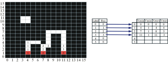
For example, consider the image in Figure 7. This is a simple 16 × 16 pixel image that contains two blobs that should be labeled by the labeling algorithm. As the algorithm begins as shown in Figure 7(a), the first three pixels encountered are labeled with new labels as they have no labeled neighbors that have been encountered yet. The pixels that are marked with red indicate special case, and a new label is used. The Record Table to the right shows the values it would take at this point in the scan of the image. Figures 7(b) and (c) show what happens when labels 1 and 2 meet and when labels 2 and 3 meet. The yellow box shows the window the algorithm is considering at that point in time. When two labels meet, the label table is updated to point to the lower record entry. This entry is also updated so that the points it describes encompass all the pixels of both labels. In this way this information is carried along. When labels 2 and 3 meet, label table 3 is made to point to record 1 also and record 1 is updated to encompass label 3’s pixels. This way the algorithm encompasses all the pixels of each pixel grouping. Figure 7(d) shows the fully labeled image with its completed record table.
3.5. Candidate Scaling
During the Labeling portion of the algorithm, contiguous pixel groupings are identified. These groupings are candidate traffic signs. Not all of these will be good candidates; many will simply be too small to contain enough information. These candidates are filtered to remove ones that do not contain enough resolution to match a traffic sign template. The remaining candidates are considered good candidates. Since the matching algorithm discussed in the next section requires that the template and the candidate images both be of the same resolution, these remaining candidates must next be scaled to match the template images resolution. Once the candidate is scaled to match the resolution of the traffic sign templates, they are subjected to the template matching portion of the algorithm.
3.6. Template Matching
Template Matching is the portion of the algorithm that takes candidates found in the previous steps and compares them with images of known good traffic signs. These traffic sign images will comprise the template library. Each potential traffic sign will be compared with each member of the template library and, if a close match is found, it is declared to be that traffic sign. This template
 (a)
(a)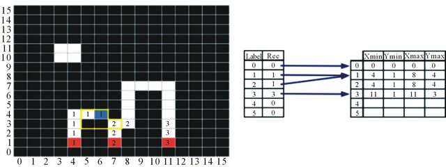 (b)
(b)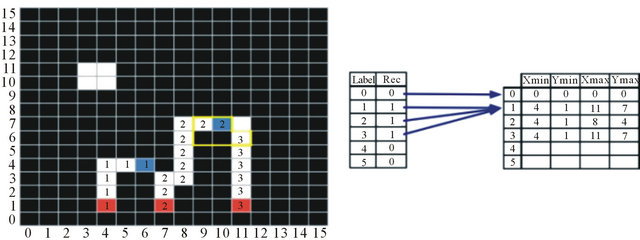 (c)
(c) (d)
(d)
Figure 7. Labeling algorithm example. (a) Initial Labeling and Record table; (b) Labeling and Record table when Labels 1 and 2 meet; (c) Labeling and Record table when Labels 2 and 3 meet; (d) Completed Labeling (Labels 1-3 all point to the same segment).
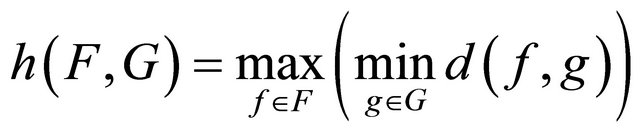
matching is done by calculating the Hausdorff distance between the candidate and each template. The Hausdorff distance calculation is a method and metric used to compare two binary image shapes. A benefit over other comparison methods is that does not rely on explicit point correspondence measuring proximity rather than exact superposition [23]. The Hausdorff distance is defined as [24]:
Given two non-empty finite sets of points
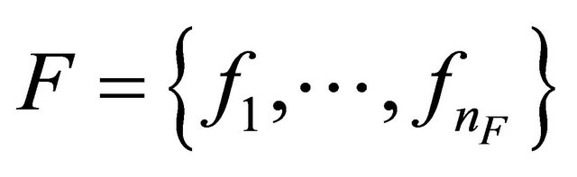 and
and 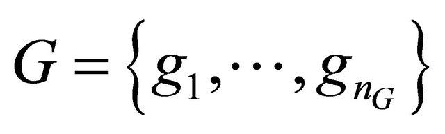 of
of and an underlying distance d, the Hausdorff distance is given:
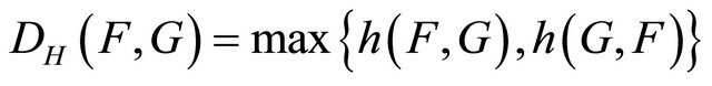 (1)
(1)
where
 (2)
(2)
If two binary images are considered to each be a set of points, then this definition essentially describes an algorithm that for each pixel of the first set will calculate the minimum distance between that pixel and every pixel in the second set. A minimum distance is also calculated for each pixel of the second image with relation to every pixel of the first image. The maximum of these minimums is the Hausdorff distance. In other words, it is a measurement of the most out-of-place pixel. This distance calculation technique has been successfully applied in other image recognition applications such as face recognition and object matching [25].
There are other approaches that can be used for this step in the overall algorithm. Several have shown good success in a variety of applications especially in contexts where the candidates may be shifts or tilts of the template. Neural Networks can be used to create a cascade of classifiers that will allow for very fast sign detection [26]. However, the process of teaching a neural network is a long one; on the order of days. Therefore, building classifiers for multiple signs become a time prohibitive approach [27]. Other possible methods for traffic sign identification use interest point correspondence to find matches. One such approach is SURF or Speeded Up Robust Features [28]. SURF makes use of 2D Haar wavelet responses to find these points of interest [29]. Various applications of SURF have been shown to be fast and robust to image transformations. Since the main objective is a practical hardware implementation, Hausdorff distance calculation was used in this work.
4. Hardware Implementation
4.1. Environment
To implement this design, a Xilinx FPGA platform and toolkit was chosen. The hardware selected was Digilent’s Virtex-5 OpenSPARC Evaluation Platform, Xilinx XUPV5-LX110T, which is a version of the ML505 Xilinx evaluation board with a larger version of the Virtex 5 FPGA. This is a versatile board with many on-board peripherals that allow for a diverse number of applications. To develop for this platform, Xilinx’s Embedded Development Kit (EDK) was used [29]. EDK enables the quick creation of an on-chip embedded processor (MicroBlaze) and user specific logic (peripherals) on a Field Programmable Gate Array (FPGA). EDK allows for strategic decisions regarding the partitioning of hardware and software implementation. Although software run time is often slower than hardware implementation, there are tasks that may be simpler to accomplish in software.
4.2. System Overview
The testing system included a Intel PC and the Xilinx XUPV5-LX110T which implements a MicroBlaze processor that uses external SDRAM memory and the image processing IP peripheral. The PC ran a custom application that opened BMP images and transferred the RGB data to the MicroBlaze over a serial UART connection. The MicroBlaze received this image data, stored it to RAM and transferred it in turn to the hardware peripheral. The hardware IP peripheral processed the image and returned it to the MicroBlaze. After highlighting any traffic signs that were found, the original image was transferred back to the PC. The MicroBlaze also used a second UART connection used for debugging and reporting.
Figure 8 shows a flowchart for the design. Here, the operational flow of the system is described in its entirety. It can be noted that each subsystem (PC, MicroBlaze, and IP peripheral) fulfills key portions of the work required. The application running on the PC is concerned with preparing the image RGB data, sending it to the embedded system, receiving it back after it has been processed, and writing it back to the file system. The MicroBlaze, in turn, receives this RGB image data, stores it, transfers it to the IP peripheral, receives it from the IP peripheral after processing, and finishes processing it before returning an updated image back to the PC. The IP peripheral receives the image data and processes it according to the algorithm steps and returns it to the MicroBlaze.
An image resolution of QVGA or quarter VGA of 320 × 240 pixels was chosen for implementation. This choice was made because it is large enough for images to contain enough information to process, but small enough to not become a limiting factor during development. The following sections describe the implementation of the key five algorithm steps as they are shown in Figure 9.
4.3. Hue Calculation and Detection
Hue calculation involves taking the stream of pixels in
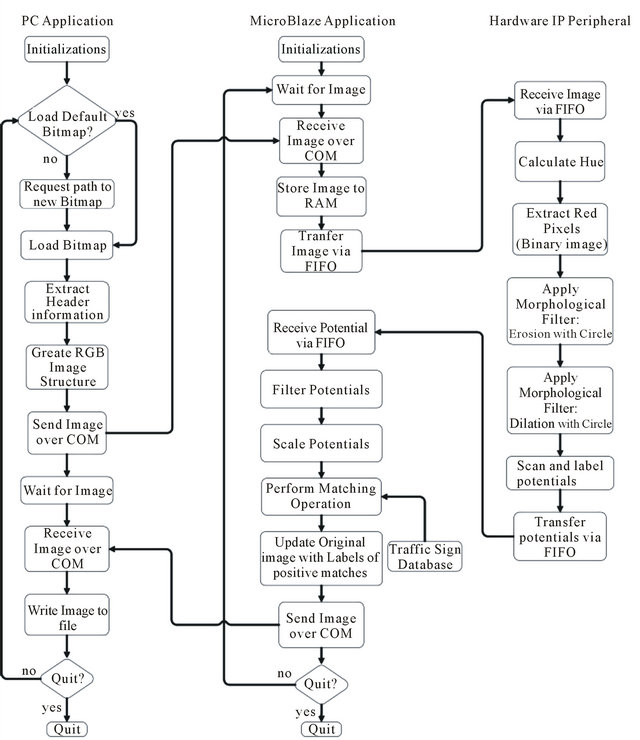
Figure 8. System flow chart.
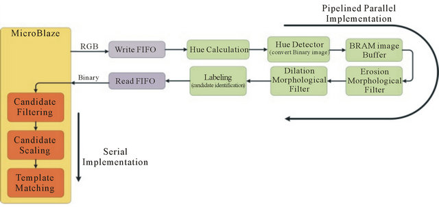
Figure 9. Image processing algorithm implementation.
RGB format and determining which pixels are red. As it was described in the previous chapter, this is done by converting the RGB triplet into a different representation of the color spectrum called HSV. However, it should be noted that one byte of this new triplet contains all the information we need.
Hue indicates that the pixel is red, the Saturation indicates where it lies between the lightest pink and solid red, and Value indicates where it lies between the darkest red and solid red. Therefore, the Saturation and Value components do not need to be calculated. Given this simplification, Figure 10 shows the implementation in hardware. This circuit accepts the RGB values and calculates the representative hue value. Most of the circuit is combinatorial. The division, however, introduces the need to add some pipelining. The division requires 17 clock cycles to fill the pipeline, but afterwards will calculate a new quotient every clock cycle. This fact required the introduction of a delay register that would allow the control signals, offsets, and quotient to align. The Hue value is taken as an angle, meaning that it takes a value between 0 and 359. This 360-degree range is normally divided into sextants representing Magenta, Red, Yellow, Green, Cyan, and Blue. These sextants then, cover a range of 60 degrees each. To simplify calculation, this implementation used sextants with a range of 0 to 63.
This resulted in a color wheel with an angle range between 0 and 383 [22]. In addition, the normal color wheel has red at the 0 angle. To avoid modulo calculation for red pixels, the color wheel was rotated in this implementtation. Magenta, a much less likely color to find in nature, was placed at the origin.
The Hue detection portion of the algorithm involves taking the stream of hue values and categorizing them as red or not-red. Given the adjusted color wheel described above, red is centered at value 64. Therefore the range within which each pixel, P, must fall is (48 ≤ P ≤ 80). As pixels are categorized, the resulting stream is binary. Figure 11(a) shows an example image and Figure 11(b) shows how this image has been converted to a binary image. This second image contains only pixels that were detected to be of a red hue.
4.4. Morphological Filtering
To implement morphological filtering, a pixel must be compared to its neighbors. Given that the image data arrives one pixel at a time, structures must be created to buffer enough pixels that will allow for these comparisons. These buffers will create a window. The center of the window is the pixel under evaluation and the other pixels in the window will contribute to whether this pixel is output as or active inactive. In this design, a 5 × 5 window was chosen. In addition to this window, a BRAM (Block RAM) buffer was used to guarantee the arrival to all pixels to be at consecutive clock cycles. The FIFO
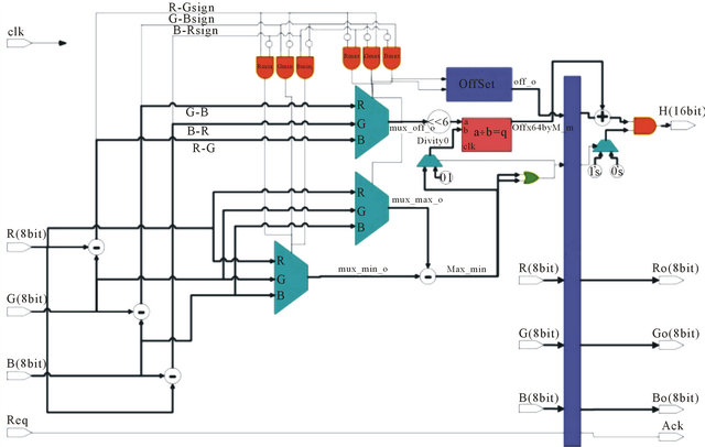
Figure 10. Hue calculator.
 (a)
(a)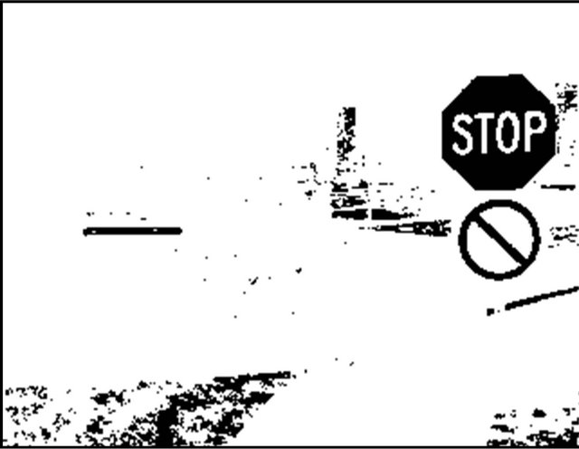 (b)
(b)
Figure 11. Results of Hue detection (red). (a) Original test image; (b) Image after detecting Red Hue.
structures linking the MicroBlaze and the IP peripheral do not send a solid stream of pixels and these breaks will affect the outcome of the morphological filtering.
Using a 5 × 5 window means that the algorithm is considering pixels from 5 different rows of the image. To allow for this, row buffers are used. A row buffer holds all the pixels in a given row to make them available when they are needed. Single bit registers were used to hold the pixels within the window. Combinational logic compares the structural element to the contents of the window and decides if the output pixel should be active or inactive.
Figure 12 shows the block diagram for the morphological filter circuit. This implementation can be used for both erosion and dilation exploiting the fact that they are duals of each other. Additionally the structural element is programmable. This allows for reuse when multiple passes are desired as in the case of combining erosion and dilation to perform an open or close operation. This flexibility proved to be very helpful when testing to identify the combination of operations that best filtered the image. A structural element of a 3 × 3 disk and a single open operation were shown to best clean up the image while not harming the traffic signs. The first step, erosion, would serve to eliminate many of the stray pixels completely and the second dilation step would serve to repair any undesired degradation to the larger pixel clusters that may be traffic signs. When the resolution of the images
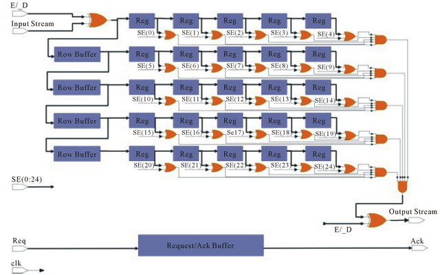
Figure 12. Morphological filter implementation with FPGA.
being processed is increased, larger structural elements may be needed to do adequate filtering.
Figure 13 shows the effect of performing morphological filtering on the test image after hue detection. The number of extraneous pixels has been greatly reduced from those in Figure 11(b). This prepares the image for the next step in the algorithm; Labeling.
4.5. Labeling
Similar to the morphological filtering, labeling requires a window where a pixel’s neighbors are observed. This window includes 5 pixels, the one current pixel and its 4 previously visited neighbors. A row buffer is needed to hold the labels of previously visited pixels until they come back into the window. Figure 14 shows the block diagram for the labeling circuit. A Label Table and Record Table are used to store the bounding box coordinates for each label. As the pixels and their labels fill the window, the update logic evaluates what the current pixels label should be and how to update the Label Table and Record Table. These two tables are continually updated to ultimately arrive at a list of labeled pixel groupings. The Update Logic block represents a behavioral process that determines the labels for each pixel and updates the Label and Record table. Given that the current pixel is active, this logic determines if this pixel will receive a new label, if it is the meeting of two labels, or simply if it is a pixel that should receive a previous label. After this, the logic will determine how to update the Label and

Figure 13. Test image after morphological filtering.
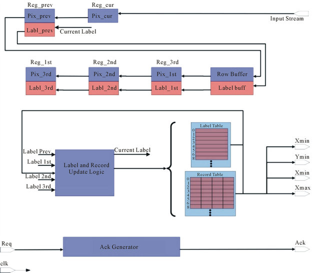
Figure 14. Labeling algorithm hardware implementation.
Record tables. New labels simple result in new entries in both tables. Pixel meetings result in Label Table entries pointing to different records as it is found that two entries should merge. Previously used labels result in the Record Table entry being grown to encompass the new pixel.
The Acknowledgement Generator (Ack) monitors the labeling process to determine when labeling is complete. This Ack signal goes high only when the Xmin, Ymin, Xmax, Ymax values become valid. For every clock cycle that this signal is high, these bounding box values indicate another labeled blob. This output is then fed back to the MicroBlaze via the FIFO for further processing. Figure 15(a) shows the test image fully labeled. At this point these are the candidates to be considered for traffic sign matching.
However if a simple filter is implemented this number of candidates is greatly reduced. By ignoring bounding boxes that have at least one dimension smaller than a specified threshold most of the candidates are rejected. It was experimentally found that a blob smaller than 16 × 16 pixels would not contain enough information to provide a good chance for any match. Figure 15(b) shows the test image after this simple filter is applied. Only 3 candidates remain. These 3 candidates will be the only ones considered during the scaling and matching steps.
4.6. Candidate Resizing
The last two algorithm steps are implemented in software running on the MicroBlaze CPU. At this point in the image processing algorithm, each traffic sign candidate must be extracted from the binary image, scaled to a resolution that will match that of the template images, and then compared to existing templates. To extract the candidate, the bounding box is passed to a routine that uses these boundaries as the edges of an image. The resulting extracted image is then scaled according to the ratio of its length and width to the length and width of the template images. The initial resolution chosen for the templates was 160 × 160 pixels.
The scaling algorithm calculates the ratio between the original size of the candidate and the template size by calculating an integer portion and a fractional part. This avoids the use of floating point arithmetic. A new memory location is used as the storage location of the new resized candidate. The algorithm scans the original size candidate and sets the pixels of the scaled candidate to active or inactive according to calculated ratios. Figure 16 depicts the extraction of the candidate from the binary image and its scaling to match the template size.
4.7. Template Matching
Template Matching involves comparing each of these scaled candidates to the library of template images. As
 (a)
(a)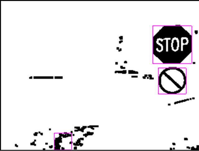 (b)
(b)
Figure 15. Labeling results. (a) Test image after labeling; (b) Test image after rejection of small labels.
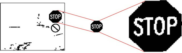
Figure 16. Extraction and scaling of candidate sign.
explained in Section 3, this comparison is done by calculating the Hausdorff distance between the candidate and the template images. Figure 17 shows some of these template images for red color.
The implementation of the calculation of the Hausdorff distance is done according to the description of the algorithm in the previous section. For each active pixel at location (x,y) of the scaled candidate image, the same pixel location of the template image is examined. If the same (x,y) location of the template image contains an active pixel that the distance between that pixel and the template is 0. If it is not an active pixel, then a search begins for the nearest active pixel. This search is conducted with an increasing radius. When an active pixel is found, the radius is the distance between that pixel of the candidate image and the template. No more distances need to be calculated for that same pixel since all other distances will be equal or greater.
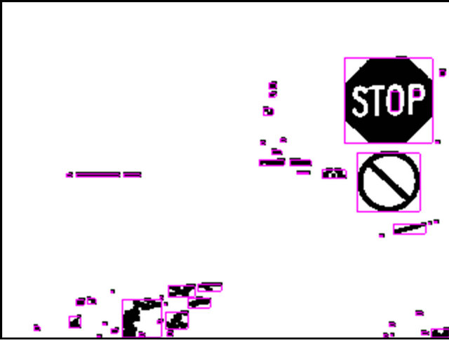
Once a Hausdorff distance is calculated for each template, they can be compared to determine if there is a good match. It was observed that at times there were high outliers and at times there was very little margin between the lowest and the next lowest value. It was determined experimentally that if a the minimum distance is found to be at least 10% lower than the average of the lowest three distances, this can be considered a good match. Because shifting to the right by 3 bits is a simpler calculation than dividing by 10, 12.5% was used instead of 10%. This method avoided the impacts of high valued outliers and clusters of low values. This provides a threshold to show that the lowest distance is actually significantly lower than the other values. If this threshold is not met, then no match is found and the image is declared to not contain any traffic signs. Figure 18 shows the test image with all 3 good candidates highlighted. The two highlighted in magenta are the candidates that found matches according to the description above. The blue highlighted candidate did not find an adequate match.
5. Results
5.1. Device Utilization
Table 1 details the usage statistics of this design implemented on the Virtex 5 device xc5vlx110t with package ff1136 and a speed grade of –1.85% of slices have been used, but very little of the fabric RAM and DSPs have been used.
5.2. Performance: Timing
The key requirement for a traffic sign recognition system is that it should operate in real-time. Depending on the application, real-time may be defined very differently. The term real time refers to a system that is able to take
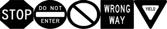
Figure 17. Template images.

Figure 18. Test image after template matching.
data and process it sufficiently rapidly to be able to take the actions required of the system. For a system, whose purpose is to detect traffic signs while traveling on the road, a threshold for real time could be calculated as the time required for detecting a sign in 50 feet of travel at 65 mph. This time is 525 milliseconds. Therefore, a system of this nature can be considered real time if it can reliably detect a traffic sign in approximately half a second.
Initially the template images were set to a resolution of 160 × 160 pixels. The candidates would then also be scaled to this size. This resolution was chosen because it was large enough to contain a good amount of detail. Table 2 shows the timing results of this system. The IP peripheral includes the all the algorithm steps that were implemented in the reconfigurable hardware namely, Hue Calculation and Detection, Morphological Filtering, and Candidate Labeling.
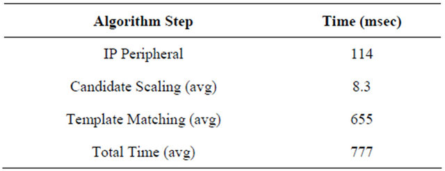
The timing shown here would likely not be adequate for the use case of the system designed here. It is clear, however, that the bulk of the time is contributed by the template matching part of the algorithm. The resolution of the templates and scaled candidates have a direct impact on this figure. Tables 3 and 4 show the results after reducing the resolution of these templates to 80 × 80 pixels and then 40 × 40 pixels. The performance improvement is dramatic.
With these substantial improvements, results are on the same order of magnitude of the goal. With an average detection time of 777 milliseconds a car could travel at 44 miles per hour and still detect a traffic sign in 50 feet.
Table 1. FPGA device utilization summary.
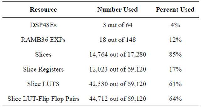
Table 2. Algorithm performance details with 160 × 160 pixel templates.
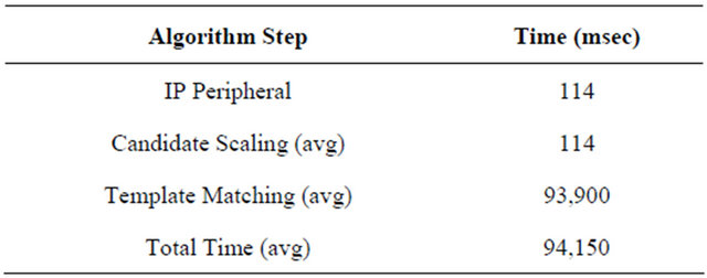
Table 3. Algorithm performance details with 80 × 80 pixel templates.
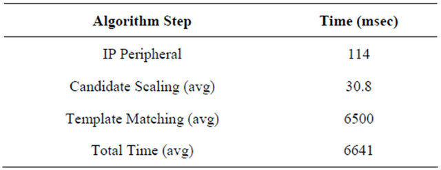
Table 4. Algorithm performance details with 40 × 40 pixel templates.
Given that the algorithm steps of Hue Calculation, Hue Detection, Morphological Filtering, and Labeling were done in the IP peripheral in only 114 milliseconds, whereas the Template Matching step, on the other hand, implemented in software running on a 100Mhz CPU, could only be performed in 655 milliseconds at best, it is clear that the parallel implementation significantly outperforms the serial software implementation.
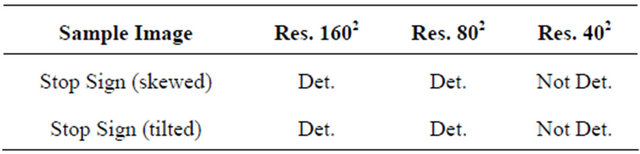
5.3. Performance: Accuracy
An important factor to the accuracy of the system is the orientation of the traffic signs with reference to the camera. When signs are perpendicular to the viewer, the system detection performance is very accurate as shown in Table 5, even with the low resolution template. If the sign is skewed or tilted, the performance could be affected. To evaluate how sensitive this system was to these perturbations, images were processed that contained them. Figure 19 shows an image similar to the one used in previous examples, but with the traffic signs at an angle to the viewer. Figure 20 is an example where the traffic signs are tilted with respect to the viewer. Table 6 details the results of processing these two example images. The stop sign is detected successfully in both of the higher resolution template versions but not with the lowest resolution.
6. Conclusion
Automotive technologies continue to explore new ways to keep drivers safe. Recently, technologies have emerged that monitor more complex parameters. This paper describes one such system. The implementation of the traffic sign recognition system uses Xilinx’s EDK toolkit to

Figure 19. Test image with skewed signs.
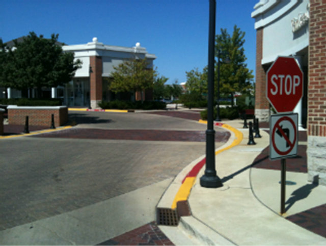
Figure 20. Test image with tilted signs.
Table 5. Algorithm accuracy.
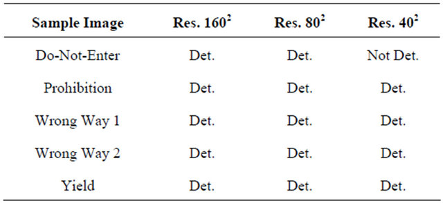
Table 6. Algorithm robustness.
create an image processing flow that is partitioned across hardware and software. An embedded processor is used to receive RGB pixel data from a PC and to forward it to a hardware IP peripheral. This peripheral in responsible for extracting red pixels, cleaning up the resulting binary image, and labeling possible candidates for matching to traffic sign templates. These candidates are passed back to the embedded processor where they are scaled and evaluated against an array of template images. The implementation described here is able to detect the sings within 50 feet of distance at a travel velocity of 44 miles per hour or less.
REFERENCES
- J. Urry, “The ‘System’ of Automobility,” Theory, Culture & Society, Vol. 21, No. 4-5, 2004, pp. 25-39. doi:10.1177/0263276404046059
- E. Eckermann, “World History of the Automobile,” Society of Automotive Engineers, Warrendale, 2001. doi:10.4271/R-272
- “Transportation: Motor Vehicle Accidents and Fatalities,” The 2012 Statistical Abstract, US Census Bureau, Suitland, 2011.
- “Population,” The 2012 Statistical Abstract, US Census Bureau, Suitland, 2011.
- “EuroFOT Study Demonstrates How Driver Assistance Systems Can Increase Safety and Fuel Efficiency,” EuroFOT, 2012. http://www.eurofot-ip.eu/en/news_and_events/eurofot_study_demonstrates_how_driver_assistance_systems_can_increase_safety_and_fuel_efficiency_acr.htm
- M. Meuter, C. Nunn, S. M. Gormer, S. Muller-Schneiders and A. A. Kummert, “A Decision Fusion and Reasoning Module for a Traffic Sign Recognition System,” IEEE Transactions on Intelligent Transportation Systems, Vol. 12, No. 4, 2011, pp. 1126-1134. doi:10.1109/TITS.2011.2157497
- C. Lai, “An Efficient Real-Time Traffic Sign Recognition System for Intelligent Vehicles with Smart Phones,” Proceedings of 2010 International Conference on Technologies and Applications of Artificial Intelligence, Hsinchu, 18-20 November 2010, pp. 195-202. doi:10.1109/TAAI.2010.41
- V. Andrey, “Automatic Detection and Recognition of Traffic Signs Using Geometric Structure Analysis,” Proceedings of SICE-ICASE International Joint Conference, Busan, 18-21 October 2006, pp. 1451-1456. doi:10.1109/SICE.2006.315823
- D. Soendoro and I. Supriana, “Traffic Sign Recognition with Color-Based Method Shape-Arc Estimation and SVM,” Proceedings of 2011 International Conference on Electrical Engineering and Informatics, Bandung, 17-19 July 2011, pp. 1-6. doi:10.1109/ICEEI.2011.6021584
- Y. Liu, H. Yu, H. Yuan and H. Zhao, “Real-Time Speed Limit Sign Detection and Recognition from Image Sequences,” Proceedings of 2010 International Conference on Artificial Intelligence and Computational Intelligence, Shenyang, 23-24 October 2010, pp. 262-267. doi:10.1109/AICI.2010.62
- R. Kastner, T. Michalke, T. Burbach, J. Fritsch and C. Goerick, “Attention-Based Traffic Sign Recognition with an Array of Weak Classifiers,” Proceedings of 2010 IEEE Intelligent Vehicles Symposium, San Diego, 21-24 June 2010, pp. 333-339. doi:10.1109/IVS.2010.5548143
- M. A. Souki, L. Boussaid and M. Abid, “An Embedded System for Real-Time Traffic Sign Recognizing,” 3rd International Design and Test Workshop, IDT 2008, Monastir, 20-22 December 2008, pp. 273-276.
- M. Muller, A. Braun, J. Gerlach, W. Rosenstiel, D. Nienhuser, J. M. Zollner and O. Bringmann, “Design of an Automotive Traffic Sign Recognition System Targeting a Multi-Core SoC Implementation,” Design, Automation & Test in Europe Conference and Exhibition (DATE), Dresden, 8-12 March 2010, pp. 532-537.
- H. Irmak, “Real Time Traffic Sign Recognition System on FPGAs,” M.S. Thesis, Middle East Technical University, Ankara, 2010.
- Frost & Sullivan, “Development of Low-cost DAS Technologies to Help Reach European Union’s Target to Increase Road and Driver Safety,” 2011. http://www.frost.com/prod/servlet/press-release.pag?docid=251082001
- Continental AG, “MFC 2 Multi-Function Camera,” Datasheet, 2009. http://www.conti-online.com/generator/www/de/en/continental/industrial_sensors/themes/mfc_2/mfc_2_en.html
- Continental AG, “Traffic Sign Recognition,” 2012. http://www.conti-online.com/generator/www/de/en/continental/automotive/general/chassis/safety/hidden/verkehrszei chenerkennung_en.html
- J. Markoff, “Smarter than You Think: Google Car Drives Itself,” The New York Times, October 2010. http://www.nytimes.com/2010/10/10/science/10google.html?_r=1
- A. C. Clark and E. N. Wiebe, “Color Principles—Hue, Saturation and Value,” North Carolina State University, Raleigh, 2002. http://www.ncsu.edu/scivis/lessons/colormodels/color_models2.html
- D. M. Rouse and S. S. Hemami, “Quantifying the Use of Structure in Cognitive Tasks,” Proceedings of SPIE, Vol. 6492, Human Vision and Electronic Imaging XII, 649210, San Jose, 12 February 2007. doi:10.1117/12.707539
- J. P. Serra, “Image Analysis and Mathematical Morphology,” Academic Press, Inc., Orlando, 1983.
- D. G. Bailey, “Design for Embedded Image Processing on FPGAs,” Wiley-IEEE Press, Singapore, 2011. doi:10.1002/9780470828519
- S. Mignot, “A Hardware-Oriented Connected-Component Labeling Algorithm,” Technical Report, GEPI—Observatoire de Paris, Paris, 2006.
- J. Chen, M. K. Leung and Y. Gao, “Noisy Logo Recognition Using Line Segment Hausdorff Distance,” Pattern Recognition, Vol. 36, No. 4, 2003, pp. 943-955. doi:10.1016/S0031-3203(02)00128-0
- E. Baudrier, F. Nicolier, G. Millon and S. Ruan, “BinaryImage Comparison with Local-Dissimilarity Quantification,” Pattern Recognition, Vol. 41, No. 5, 2008, pp. 1461- 1478. doi:10.1016/j.patcog.2007.07.011
- C. Y. Fang, S. W. Chen and C. S. Fuh, “Road-Sign Detection and Tracking,” IEEE Transactions on Vehicular Technology, Vol. 52, No. 5, 2003, pp. 1329-1341. doi:10.1109/TVT.2003.810999
- M. F. Hashim, P. Saad, M. R. M. Juhari and S. N. Yaakob, “A Face Recognition System Using Template Matching And Neural Network Classifier,” Proceedings of 1st International Workshop on Artificial Life and Robotics, Kangar, May 2005, pp. 1-6.
- H. Bay, A. Ess, T. Tuytelaars and L. Van Gool, “SpeededUp Robust Features (SURF),” Computer Vision and Image Understanding, Vol. 110, No. 3, 2008, pp. 346-359. doi:10.1016/j.cviu.2007.09.014
- “Embedded System Tools Reference Manual EDK (v 13.2),” Xilinx, 2011. http://www.xilinx.com/support/documentation/sw_manuals/xilinx13_2/est_rm.pdf