Journal of Signal and Information Processing
Vol.4 No.3(2013), Article ID:35350,14 pages DOI:10.4236/jsip.2013.43031
Time-Varying Bandpass Filter Based on Assisted Signals for AM-FM Signal Separation: A Revisit*
![]()
1Ocean Department of Dalian Naval Academy, Dalian, China; 2Navgation Department of Dalian Naval Academy, Dalian, China.
Email: xgl_86@163.com
Copyright © 2013 Guanlei Xu et al. This is an open access article distributed under the Creative Commons Attribution License, which permits unrestricted use, distribution, and reproduction in any medium, provided the original work is properly cited.
Received June 2nd, 2013; revised July 5th, 2013; accepted July 13th, 2013
Keywords: Time-Varying Bandpass Filter (TVBF); Hilbert Tranform; Assisted Signal; AM-FM Component; Time-Frequency Distribution (TFD)
ABSTRACT
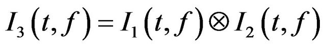
In this paper, a new signal separation method mainly for AM-FM components blended in noises is revisited based on the new derived time-varying bandpass filter (TVBF), which can separate the AM-FM components whose frequencies have overlapped regions in Fourier transform domain and even have crossed points in time-frequency distribution (TFD) so that the proposed TVBF seems like a “soft-cutter” that cuts the frequency domain to snaky slices with rational physical sense. First, the Hilbert transform based decomposition is analyzed for the analysis of nonstationary signals. Based on above analysis, a hypothesis under certain condition that AM-FM components can be separated successfully based on Hilbert transform and assisted signal is developed, which is supported by representative experiments and theoretical performance analysis on error bound that is shown to be proportional to the product of frequency width and noise variance. The assisted signals are derived from the refined time-frequency distributions via image fusion and least squares optimization. Experiments on man-made and real-life data verify the efficiency of the proposed method and demonstrate the advantages over the other main methods.
1. Introduction
The decomposition of signals blended in noises is a reallife problem in measurement and other signal processing fields, which includes two tasks: first filtering and then decomposing the signals. The filtering of signals from observed noisy data, while preserving their original features respectively, remains a challenging problem in both signal processing and statistics. A number of filtering methods have been proposed, particularly for the case of additive white Gaussian noise [1-10]. Frequently, linear methods such as the Wiener filtering [1,4,10,11] are used because linear filters are easy to design and implement. However, linear filtering methods are not very effective when signals are nonstationary. To overcome the shortcomings, nonlinear methods have been proposed such as wavelet thresholding [5,7]. The idea of wavelet thresholding relies on the assumption that signal magnitudes dominate the magnitudes of the noise in a wavelet representation so that wavelet coefficients can be set to zero if their magnitudes are less than a predetermined threshold [1,7]. A limit of the wavelet approach is that the basis functions are fixed and, thus, do not necessarily match all real signals. On the other hand, the second task—the decomposition of multi-components is also an important problem in signal processing. The adaptive methods for signal separation should be explored [2,8-18] especially for the separation of multiple components blended in noise data. That is to say, the separation of signals from real-life observed noisy data include two steps’ work, filtering the signals and then decomposing the signals to multiple independent components. In most of the reported papers [1-25], the two tasks are separate and they cannot do the both tasks at the same time. In this paper, we will combine these two tasks to single one.
Among many types of signals, the AM-FM (amplitude modulation and frequency modulation) signals are one of the most important ones and play an important role in various signal processing fields [1]. In telecommunications, amplitude modulation and frequency modulation convey information over a carrier wave by varying its instantaneous amplitude and frequency. AM-FM signals are also widely used in telemetry, radar, seismic prospecting and newborn EEG seizure monitoring, broadcasting music and speech, two-way radio systems, magnetic tape-recording systems and some video-trans-mission systems. Furthermore, many real-life signals can also be taken as the AM-FM signals approximately. In some cases, once the multiple AM-FM components are superposed and noised, the information carried by every AM-FM component is blended and hidden and cannot be recognized clearly. In this work, an elementary fundamental problem how to separate the AM-FM components blended in noises is addressed.
There have been some methods involving decomposing the superposed AM-FM components, including the frequency domain separation method such as the LFM (linear frequency modulation) component separation via FRFT [17], the empirical mode decomposition (EMD) [3,12], the improved EMD (IEMD) [2,8] (the method in [8] is only for pure FM signal), the masking method [13,14] and the Hilbert transform [1,19] based method [16]. The frequency domain separation method is the most traditional method to separate the superposed AMFM components in frequency domain or fractional frequency domain [17] through finding the separation points or peak points. For the case that the superposed AM-FM components have distinguishable frequency regions, the separation is done well. Unfortunately, once the superposed AM-FM components have overlapped and undistinguishable frequency regions, the separation method in frequency domain will fail to work.
After the introduction of the HHT by Huang et al. [12], the EMD has become an important tool to analyze nonlinear and non-stationary signals by breaking them down into a number of elementary amplitude and frequency modulated (AM/FM) zero mean signals termed intrinsic mode functions (IMFs). The EMD can separate the superposed AM-FM components successfully under some conditions that have been addressed by Rilling and P. Flandrin [18], i.e., when and where the two tones (can be taken as two simple AM-FM components) can be separated well using EMD. If these conditions are not satisfied, EMD fails to separate them. Therefore, the improved EMD (IEMD) method [2] for AM-FM component decomposition is proposed in order to avoid the failure of EMD. Although IEMD can improve the performance, there are still some problems. First, the IEMD method is not stable, and in some cases it fails to separate the superposed AM-FM components, e.g., the possible failure of the polynomial estimation for more complicated frequency and phase functions due to the long signal’s length. Second, the employment of this IEMD method is cumbersome for more complicated cases such as the components with crossed instantaneous frequencies.
The masking method [13,14] uses the mask signals to help decompose the superposed AM-FM components. In fact this method makes full use of the characters of filter bank for EMD [3] to extract the component whose frequency is close to the mask signal, and then eliminates the mask signal in IMFs to obtain the components. This method has two problems. The mask signal is based on Fourier spectral, therefore this method fails to handle the case of time-varying instantaneous frequencies that have overlapped frequency regions in frequency domain. In addition, this method still fails to separate two components with crossed frequencies.
Differently, the Hilbert transform based method can separate the superposed AM-FM components whose frequencies are very close in principle. Unfortunately, the frequency of the assisted signal used in the Hilbert transform based method needs to be found in the Fourier transform domain via the valley values that can distinguish the different frequency modes. In other words, in the case of more overlapping of frequencies, this method will fail.
In this paper, we will first analyze the performance of the Hilbert transform based method in great details and find its limitation, and then find its potential value for analysis of the more complicated cases such as timevarying instantaneous frequencies with overlapped and crossed points. The main aim in Section 2 to analyze the Hilbert transform based method is twofold: 1), we want to know what amplitudes and frequencies are the optimal for the assisted signals; 2), for the overlapped frequencies (e.g., the Figure 1) in Fourier transform domain, whether this method will still work well or not? After that, in Section 3, the time-varying bandpass filter based on Hilbert transform and assisted signals is proposed, in addition the error bounds are analyzed theoretically and verified via simulations. The estimation of time-varying assisted signals is addressed in Section 4 via image fusion and least square optimization. In Section 5 experiments on manmade and real-life data are shown. Section 6 concludes this paper.
2. Component Separation via Hilbert Transform and Assisted Signal
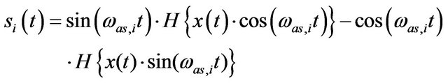
2.1. Component Separation
The decomposition theorem [16] by G. Chen and Z. Wang is defined as follows. Let  denote a real time series of n significant frequency components
( ) in
) in  of the real time variable t. It can be decomposed into n signals
  (
( ) whose Fourier spectra are equal to
over n mutually exclusive frequency ranges:
 (a)
(a)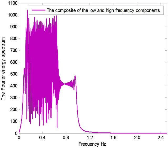 (b)
(b)
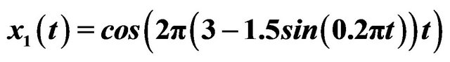
Figure 1. An example of two AM-FM components that can be separated successfully via Equations (6) and (7). Here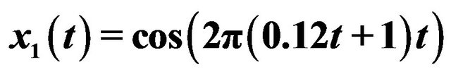 ,
,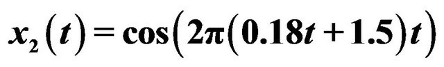 and
and ,
, . Sampling frequency is 500 Hz, time support is 30 seconds. Finally,
 .
.
 ,
, ,
, ,
, . That is,
 . (1)
. (1)
Here,  is the Fourier transform of
 ,
, ![]() represents a frequency variable, and
represents a frequency variable, and 
 are
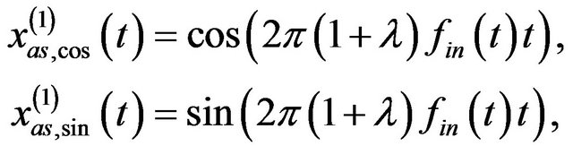
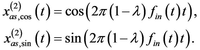
are  assisted frequencies for the assisted signals. Each signal has a narrow bandwidth in the frequency domain and can be determined by
 , (2)
, (2)
 ,(3)
,(3)
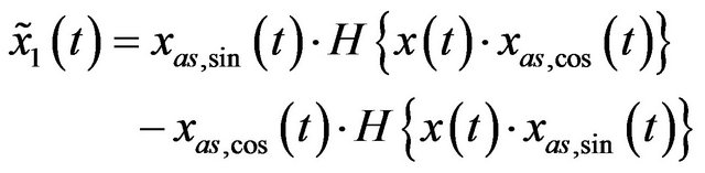
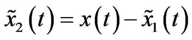
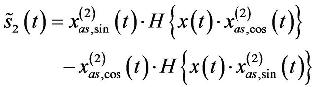
where , and H{·} represents the Hilbert transform of the function inside the bracket “{}”.
The proof of this theorem can be found in [2]. This theorem tells us two key issues: the determination of assisted signal and the condition that this theorem holds. Very fortunately we find an exciting fact: even if there are overlapped frequency ranges in Fourier transform domain, the above theorem still hold in some conditions.
Hypothesis 1: For two harmonic AM-FM components ![]() (
(![]() and
and
![]() ) in
) in![]() , if
, if ![]() and
and  are positive amplitudes, it’s possible we have
 , (4)
, (4)
 , (5)
, (5)
if  and
and  satisfy certain conditions. These conditions will be determined by rational simulations in the following section.
2.2. The Conditions for Hypothesis 1
For two harmonic AM-FM components
 and
and 
 in
in , we first assume that
  and
and  are positive amplitudes. In order to simplify our analysis, we let
![]() ,
, ![]() and the assisted signal
and the assisted signal![]() ,
, . Here
 , the circle instantaneous frequency
  is slow-varying in
 , a, c and k are constants with
 . Then we can obtain
 (6)
(6)
 . (7)
. (7)
If  and
and , then the separation is fully successful, otherwise, there is error. To measure the error quantitatively, we set
 . (8)
. (8)
Clearly, if , then the separation is fully successful. With the increasing of
![]() , the performance of decomposition will degrade. If
, the performance of decomposition will degrade. If , then the decomposition is a full failure.
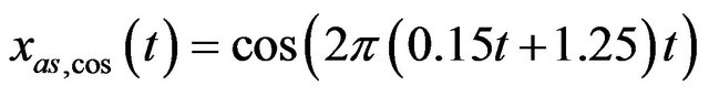
2.2.1. For  with a and c Varying
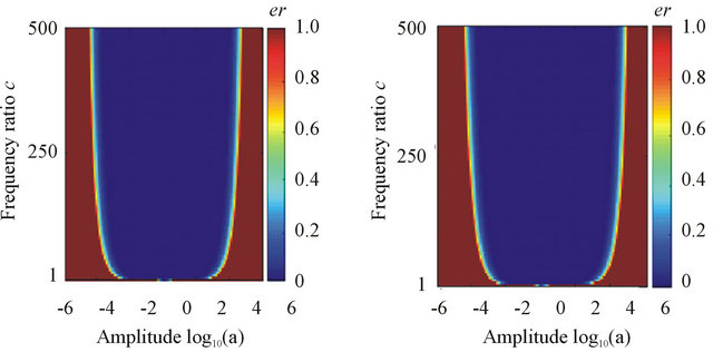
Case 1: the amplitude a changes from 10−6 to 106, and c changes from 1 to 500 and . The decomposition result can be found in Figure 2(a).
Case 2: the amplitude a changes from 10−6 to 106, and c changes from 1 to 500 and . The decomposition result can be found in Figure 2(b).
Case 3: the amplitude a changes from 10−6 to 106, and c changes from 1 to 500 and .
.
The decomposition result can be found in Figure 2(c).
Clearly, for different instantaneous frequencies (the constant frequency, the linear modulation frequency and the quadratic modulation frequency), the decompositions are the similar and we can obtain the same result: if the amplitude a and the frequency ratio c are in the blue regions in the shape of “U”, i.e., satisfy the relation
 (a)
(a)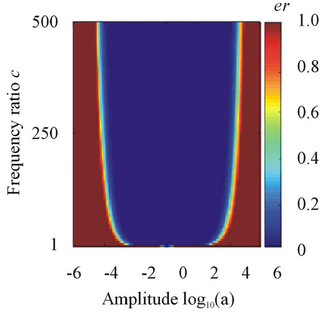 (b)
(b)
Figure 2. The separation results of different instantaneous frequencies via Equations (6) and (7).
 , then the decomposition will be nearly perfect.
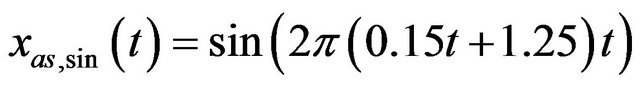
2.2.2. For c = 2 with a and k Varying
Case 1: the amplitude a changes from 10−6 to 106, and k changes from 1 to 500 and . The decomposition result can be found in Figure 3(a).
 ,
,
 and
and
 ,
,
 . Sampling frequency is 500 Hz, time support is 30 seconds. Finally,
 .
.
Case 2: the amplitude a changes from 10−6 to 106, and k changes from 1 to 500 and . The decomposition result can be found in Figure 3(b).
Case 3: the amplitude a changes from 10−6 to 106, and k changes from 1 to 500 and .
.
The decomposition result can be found in Figure 3(c).
Clearly, for different instantaneous frequencies (the constant frequency, the linear modulation frequency and the quadratic modulation frequency), the decompositions are the similar and we can obtain the same result: if the amplitude a and the frequency ratio k are in the blue regions, i.e., the middle region between the two functions
 (a)
(a)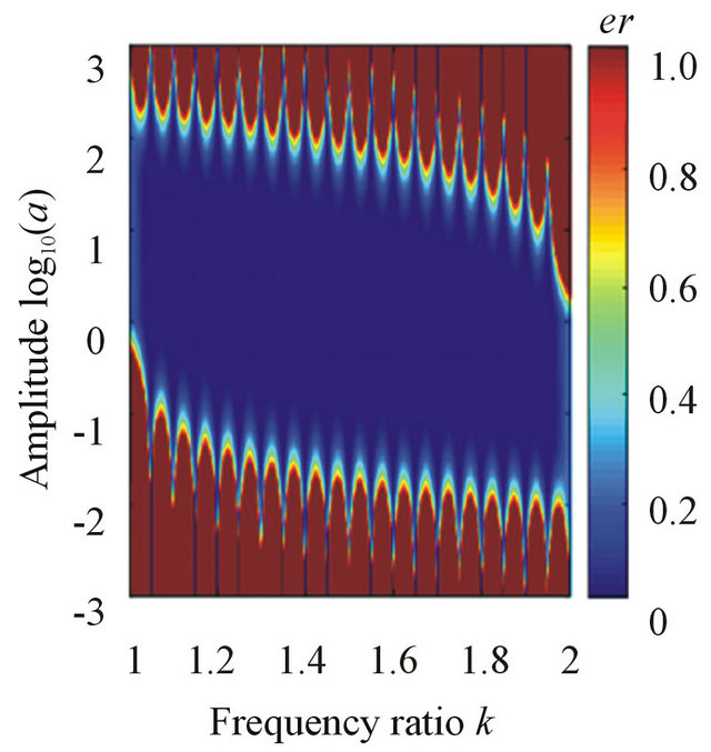 (b)
(b)
Figure 3. The separation results of different instantaneous frequencies via Equations (6) and (7).
 and
and , then the decomposition will be nearly perfect.
Therefore, if the amplitudes and frequencies of the two AM-FM components are known, the assisted signal’s frequency can be selected in wide scope according to the above results because the conditions ( , the middle region between
  and
and
 ) are very loose and easy to satisfy in practice.
The example in Figure 1 is a breakthrough of the decomposition theorem in [16]. The simulations in Figures 2 and 3 verify that this breakthrough is rational and find the performance bounds for the separation of two AMFM components.
Compared with the performance limitation of EMD [12], the method based on Hilbert transform and assisted signal is a great improvement for component separation. That is, if we can obtain the rational assisted signals, the separation of AM-FM components will be feasible in principle.
3. Time-Varying Bandpass Filter
3.1. Time-Varying Bandpass Filter
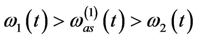
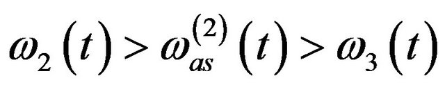
Let  with
with  denote a real time series of 3 significant instantaneous frequentcies (here the amplitude
 , and these slow-varying instantaneous frequencies satisfy
 for any
 . Now we want to obtain the interested component
  out of
 .
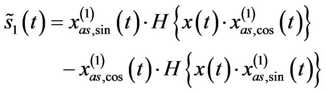
.  and
and
 are the assisted signal pairs so that
 with
with
 , (9)
, (9)
 with
with
 . (10)
Then we can obtain an approximation of the interested component  with error
 ![]() by the time-varying
by the time-varying
bandpass filter (TVBF)
 , (11)
 , (12)
 , (13)
where 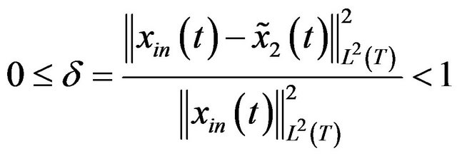 (
(![]() is a very small nonnegative value).
is a very small nonnegative value).
The most important is the selection of these functions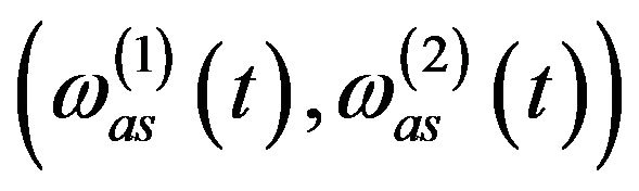 .
.
In fact, if the instantaneous frequency 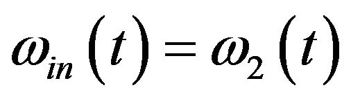 is known, we can let
 and
and 
with  only if
  and
and
 hold. If the other two components
  are the noises (such as the zeromean Gaussian white noises) whose bandwidths occupy the whole frequency domain. Therefore, we hope
 ![]() to be as small as possible. On the other hand, if
to be as small as possible. On the other hand, if ![]() is too small, the performance of TVBF in (11)-(13) will decrease because the limited signal resolution won’t be too - high for the reason of sampling and others. In the follow section, we will address the optimal
is too small, the performance of TVBF in (11)-(13) will decrease because the limited signal resolution won’t be too - high for the reason of sampling and others. In the follow section, we will address the optimal ![]() for fixed instantaneous frequency
for fixed instantaneous frequency  under different SNR
(signal-to-noise-ratio) (or noise variance![]() ).
).
3.2. Optimal Filter Parameter in Noises
In this section, we explore the optimal ![]() under different noise variance
under different noise variance ![]() for the fixed instantaneous frequency
for the fixed instantaneous frequency  via simulations. We set
 ![]() with the instanttaneous frequency
with the instanttaneous frequency ![]() (the time support
(the time support  and the sampling frequency is 500 Hz). According to (11)-(13), we set
 (14)
(14)
 (15)
(15)
Set , and
, and  is the zeromean Gaussian white noise with variance
![]() . Now we use the TVBF to obtain
. Now we use the TVBF to obtain  (an approximation of the interested component
 ) so as to see how the error
 ![]() varies while the variance
varies while the variance ![]() and the parameter
and the parameter ![]() varying.
varying.
If there are no other components whose frequencies are close to the interested component, when the noise variance is small, we can let ![]() be large. However, if there are other components whose frequencies are close to the interested component, then we must let
be large. However, if there are other components whose frequencies are close to the interested component, then we must let ![]() as small as possible. On the other hand, in order to separate the interested component,
as small as possible. On the other hand, in order to separate the interested component, ![]() cannot be zero. Therefore, after analysis and simulation in Figure 4 (see the red dot lines), we find that the optimal
cannot be zero. Therefore, after analysis and simulation in Figure 4 (see the red dot lines), we find that the optimal ![]() should be in the scope of 0.001 ~ 0.1 in most cases. Of course, in practice we should take care of all the factors comprehensively to give a better choice of
should be in the scope of 0.001 ~ 0.1 in most cases. Of course, in practice we should take care of all the factors comprehensively to give a better choice of ![]() empirically.
empirically.
Compared with the performance limitation of EMD [12], the method based on Hilbert transform and assisted signal is a great improvement for component separation. That is, if we can obtain the rational assisted signals, the separation of AM-FM components will be feasible in principle.
3.3. Performance Analysis in Noises
In follows, we will analyze the error resulted by the equivalent component that has the same frequency as the assisted signal pairs from the Gaussian noises and the middle parts between the two assisted signal pairs in the time-frequency distribution. First we set the Gaussian noise  with
with
 and
and

 , that is to say,
  is the assumed equivalent component (coming from the Gaussian noise) that has the same bandwidth as
 , and
, and  is the assumed equivalent component (coming from the Gaussian noise) that has the same bandwidth as
 .
. is the equivalent component (coming from the Gaussian noise) whose bandwidth occupies the frequency range over
 .
.  is the equivalent component (coming from the Gaussian noise) whose bandwidth occupies the frequency range less than
 .
.  is the equivalent component (coming from the Gaussian noise) whose bandwidth occupies the frequency range between
  and
and
 . Therefore
 . (16)
Taking into account (14), (15) and (16), finally we obtain
Since the bandwidth of  is the same as
  and the Gaussian white noise’s spectrum magnitude is constant, we obtain
  so that

without loss of generality, hence .
.
In the same manner, we have

Since the bandwidth of  is the same as
  and the Gaussian white noise’s spectrum magnitude is constant, we obtain
 , so that

without loss of generality, hence .
.
Finally,
 .
.
Taking into account that  is the equivalent component (coming from the Gaussian noise) whose bandwidth occupies the frequency range between
 and
and , and the Gaussian white noise’s spectrum magnitude is constant , we get
 . (17)
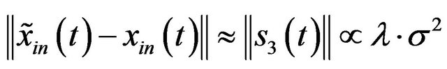
This implies that the recovery error is proportional to the value of ![]() and the variance
and the variance  of the noise. This has been verified by the simulation in Figure 4 and the two results (the theoretical result in (17) and the simulation result in Figure 4) are consistent.
4. Parameter Estimation for Assisted Signals from TFDs
4.1. Refined TFD via Image Fusion
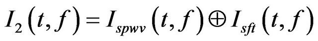
In order to obtain the assisted signals and their instantaneous frequencies, we need to obtain the refined TFD of the original signals in noises, in which we can estimate the assisted signals’ instantaneous frequencies that satisfy the relations in TVBF. In our work, we would like to use these traditional tools [1,11] such as Wigner-Ville distribution, pseudo Wigner-Ville distribution, smoothed pseudo Wigner-Ville distribution and short Fourier transform to refine our TFD by fusion rather than some updated TFDs [19,24] because these traditional but simple and reliable TFDs are enough for our task. The fusion procedure is as follow.
1) Calculate the normalized Wigner-Ville distribution , pseudo Wigner-Ville distribution
 , smoothed pseudo Wigner-Ville distribution
  and short Fourier transform
 . Here the “normalized” means that all the images above are mapped to the value scope between 0 and 1 in proportion.
2) Calculate the first refined TFD by , where
  denotes

Figure 4. Relation between the error  with the variance
 ![]() and the parameter
and the parameter .
.
(where ) by
) by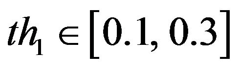 ).
).
3) Calculate the second refined TFD by
 by threshold
  (generally
 ). Additional operations: if there are many small isolated regions, then the following steps are adopted: a) perform isolated block removal whose area is less than
  (generally
 ) that is the number of the pixels in
 ; b) dilate the image
 ; c) erode the image
 .
.
4) Calculate the third refined TFD by
 , where
  denotes first performing multiplication pixel by pixel and then the following steps are possibly adopted: a) perform isolated block removal whose area is less than
  (generally
 ) that is the number of the pixels; b) dilate the image; c) erode the image.
Note that there is no normal theoretical foundation for the fusion procedure due to the complicated variants in practice. However, these thresholds and the approaches can be found in the similar context in image processing [15]. The similar empirical employment of this fusion procedure can also be found in [19,26].
We find that for most cases, the above procedure plays an effective role in refining the TFD. Figures 5-7 are three examples showing the effective results by the above procedure. Note that the refining of the TFD in our work is not our final target, which is only a basis in the process of our component separation in noises. Therefore, even we obtain the crude TFD with some distortion in our selected interested regions, if the most pixel points in the true time-frequency ridge are obtained, the effective assisted signals’ instantaneous frequencies are available via least squares optimization. For example, in Figures 5(i) and 6(i) there are some points that are not in the true time-frequency ridges, but they are distributed nearly uniformly around the true time-frequency ridges. On the other hand, our assisted signals’ instantaneous frequencies can be defined in a scope (see Figure 4) limited by ![]() that give us more tolerance for the distortion of TFD. Similarly, we can select the regions of other interested frequencies in Figures 5 and 6. These selected points
that give us more tolerance for the distortion of TFD. Similarly, we can select the regions of other interested frequencies in Figures 5 and 6. These selected points  (the red points in the image of Figures 5(i) and 6(i)) can be used to estimate the polynomial instantaneous frequency applied for the construction of assisted signals via least squares optimization.
Since the practical TFDs in noises are possibly too complicated with some intersections, it is too hard to automatically select the interested components’ regions in TFDs. Therefore, we have to artificially select our in-
 (a)
(a)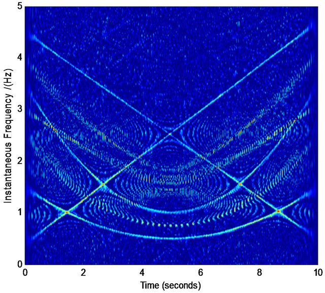 (b)
(b) (c)
(c) (d)
(d)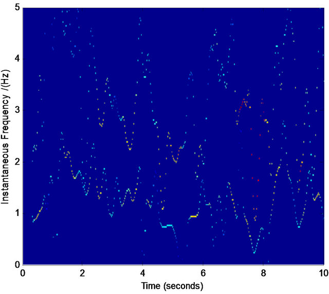 (e)
(e)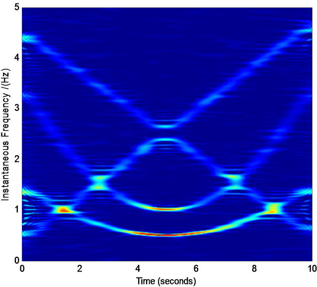 (f)
(f) (g)
(g) (h)
(h) (i)
(i)
Figure 5. Normalized TFD for assisted instantaneous frequency construction. (a) Wigner-Ville distribution; (b) pseudo Wigner-Ville distribution; (c) short Fourier transform; (d) smoothed pseudo Wigner-Ville distribution; (e) HHT; (f) the fused result of (c) and (d); (g) the fused result of (a) and (b); (h) the fused result of (f) and (g); (i) an example of the interested frequency component selection for the further estimation of assisted signal’s instantaneous frequency. Here ![]() ,
, ![]() ,
,  ,
,  ,
,  ,
, ,
,  ,
,  , and the zero-mean Gaussian noise’s variance
 . The sampling frequency is 100 Hz.
terested components via image region selection [15]. There are many powerful and skillful tools [15] to help to operate image region selection. Even in MATLAB [9], we can easily operate the image region selection piecewise via some simple tries and tests after a few times.
4.2. Polynomial Instantaneous Frequency Construction via Least Squares
We let the selected region’s instantaneous frequency be
![]() (
(![]() is the number of the coefficients).
is the number of the coefficients).
 (a)
(a)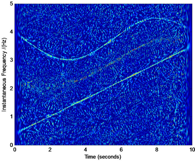 (b)
(b)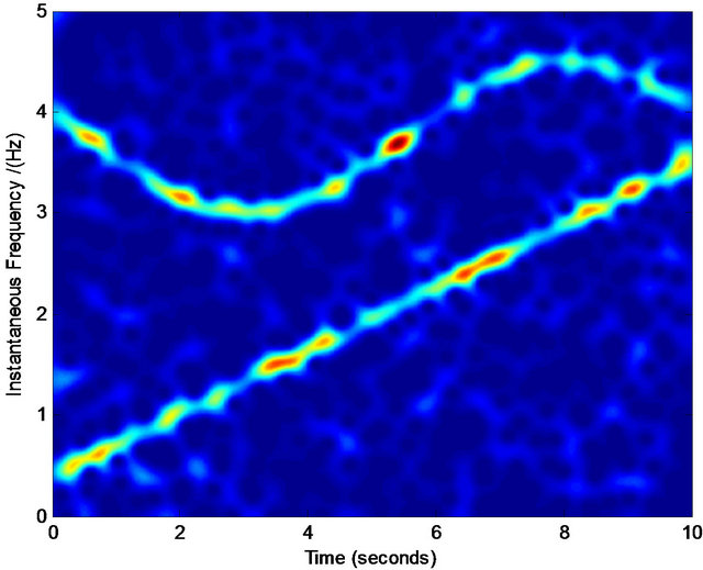 (c)
(c)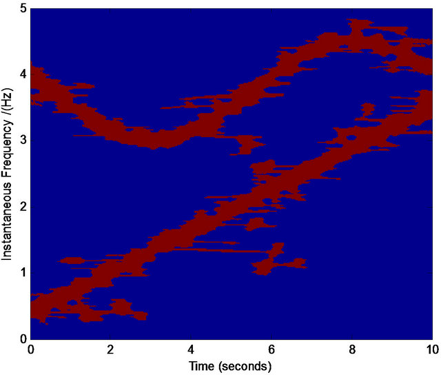 (d)
(d)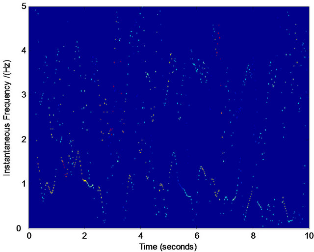 (e)
(e)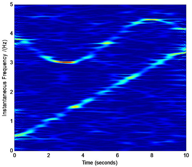 (f)
(f)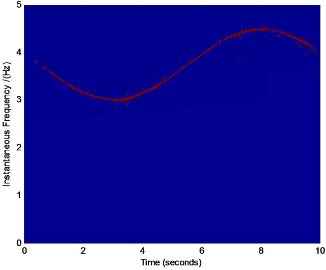 (g)
(g)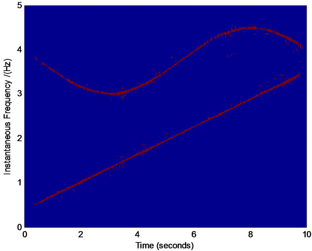 (h)
(h) (i)
(i)
Figure 6. Normalized TFD for assisted instantaneous frequency construction. (a) Wigner-Ville distribution; (b) pseudo Wigner-Ville distribution; (c) short Fourier transform distribution; (d) smoothed pseudo Wigner-Ville distribution; (e) HHT; (f) the fused result of (c) and (d); (g) the fused result of (a) and (b); (h) the fused result of (f) and (g); (i) an example of the interested frequency component selection for the further estimation of assisted signal’s instantaneous frequency. Here ,
,  ,
,  ,
,  ,
,  ∙
∙ ,
,  and the zero-mean Gaussian noise’s variance
 . Sampling frequency is 25 Hz.
From the selected region, we can obtain the nonzero pixel points  (
( and
and  is the number of the nonzero pixel points in the selected region).
Set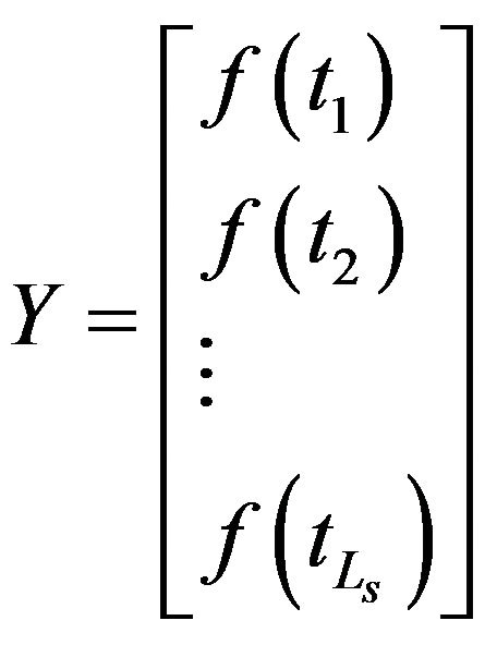 ,
, and
and , then we can obtain the optimal parameters via the least squares optimization by
 , (18)
where the superscript “![]() ” is the matrix transpose operator.
” is the matrix transpose operator.
In most cases, what we need to do is to provide the number ![]() of the parameters in
of the parameters in . In fact, after the acquisition of the refined TFD, every frequency ridge
 (a)
(a)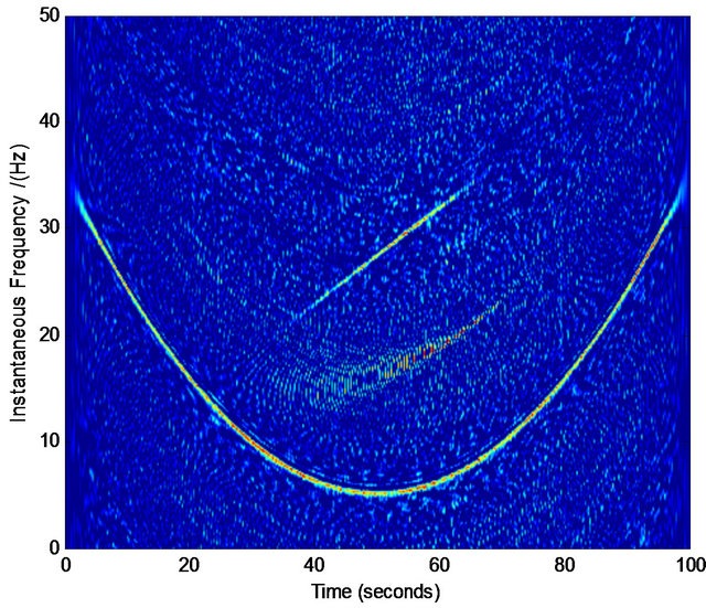 (b)
(b)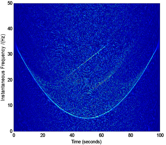 (c)
(c)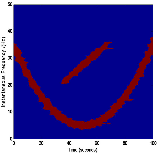 (d)
(d) (e)
(e)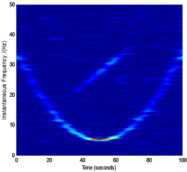 (f)
(f) (g)
(g)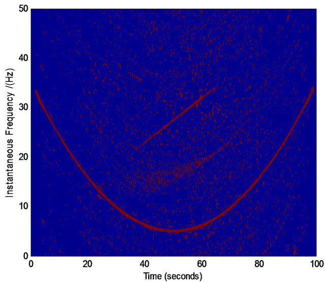 (h)
(h)
Figure 7. Normalized TFD for assisted instantaneous frequency construction. (a) Wigner-Ville distribution; (b) pseudo Wigner-Ville distribution; (c) short Fourier transform distribution; (d) smoothed pseudo Wigner-Ville distribution; (e) HHT; (f) the fused result of (c) and (d); (g) the fused result of (a) and (b); (h) the fused result of (f) and (g). Here![]() ,
, ![]() ,
, ![]() ,
, ![]() ,
, ![]() ,
, ![]() and the zero-mean Gaussian noise’s variance
and the zero-mean Gaussian noise’s variance . The sampling frequency is 250 Hz.
function’s shape is salient, and we can give a number a priori. Generally,  works well.
Once the instantaneous frequency 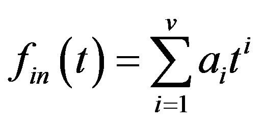 is determined, we can obtain the according two assisted signals’ instantaneous frequencies
 and
and  to construct the two assisted signal pairs:
![]() , (19)
, (19)
![]() . (20)
. (20)
Furthermore, we can obtain the according interested component’s approximation  from the noised signal
  by
by
 , (21)
 , (22)
 , (23)
and with the SNR
 , (24)
where  is the according interested original component.
In practice, the Hilbert transform has the boundary effect [1] near the endpoints that is similar with EMD’s boundary effect [20-23]. One of the most used methods [20-23] is the prolonging on the two sides of the original signals via rational extrapolation. Since there are a lot of noises, it is relatively hard to extend the original signals with seamless splicing. Therefore, in this work we use one simple but effective method: mirror extension [20]. We find that although the mirror extension cannot eliminate the boundary effect completely, it greatly attenuates the errors resulted by the boundary effect.
5. Experiments and Discussion
5.1. On Simulations
In this section, we will use the proposed method to separate the noised AM-FM components in the Figures 5-7. There are eight significant AM-FM components at all. In these experiments, we take  for all components. The compared methods include the empirical mode decomposition (EMD) [12], the improved EMD (IEMD) [2], the Hilbert transform based method [16] via Fourier spectra, the masking method [13,14] and our proposed method. In EMD we will use the most related IMF to the original true component as the according separated component. In IEMD and the masking method, we first perform simple filtering by EMD via discarding the first two IMFs. In the Hilbert transform based method [16], we assume the number of the components in noises is known so that we can obtain according modes’ number a priori. The comparison via SNR can be found in Table 1. The measure used in Table 1 is defined in (24). The signals that are decomposed come from Figures 5-7. The comparison methods are the above mentioned methods: EMD, IEMD, masking method and our proposed method.
One notation is that all the other four methods (EMD, IEMD, masking method and the Hilbert transform based method [16]) fail to separate the components with crossed instantaneous frequencies. EMD, IEMD and masking method only extract the high-frequency part every time. At the same time, they are seriously affected by the noises. The method [16] employs the Fourier spectra to obtain the assisted signals’ constant frequencies, which are not suitable for the time-varying frequency components, and in other words, it only holds for the components with distinguishable (or non-overlapped) frequency regions in Fourier spectra. Therefore, these four methods’ performance is far lower than our proposed method for the more general and complicated cases in noises.
In Figure 7, the second component  is intermittent. In this case, we still obtain the selected region including the according pixels that are related with the instantaneous frequency of
  at first. Then the construction of the assisted signals is also the same as that of
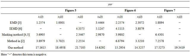
Table 1. The comparison between some methods to separate the components in noises.
non-intermittent component. The difference is the extraction of the component using TVBF. Since the component is intermittent, then its effective time support is short than the whole time support. Therefore, we only need to extract the according component in the effective time support that can be estimated in the refined TFD. In order to reduce the lose of the small instantaneous amplitude as much as possible without introducing more noises, we can extract the component by
 , (25)
where  is the component’s effective time support roughly estimated in the TFD, and here we take
 .
.
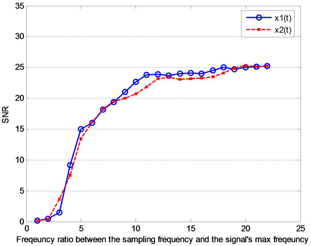
Another problem is the sampling frequency. Since Hilbert transform will be affected by the sampling frequency and the signal’s max frequency, we must take into account the ratio between the sampling frequency and the signal’s max frequency. We find that with the increasing of the ratio between the sampling frequency and the signal’s max frequency, the performance will upgrade, and vice versa. Figure 8 is the relation between the SNR and the frequency ratio for the separation of the two components from Figure 6. We find that the higher the ratio, the higher the SNR. In addition, when the ratio is more than 10, the SNR varies slowly. In the same manner, we also test the components in Figures 5 and 7 and obtain the same conclusion for fixed noise’s variance: when the ratio is more than about 10, the performance is better. On the other hand, when the ratio is more than about 5, the performance is nearly acceptable.
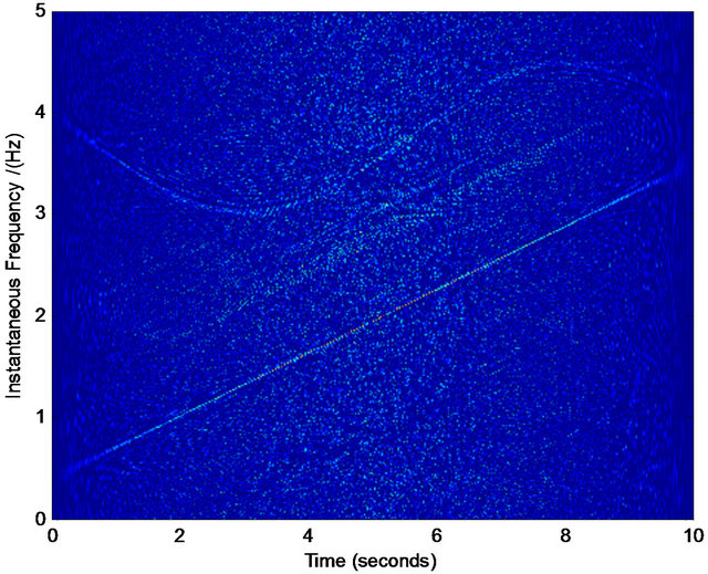
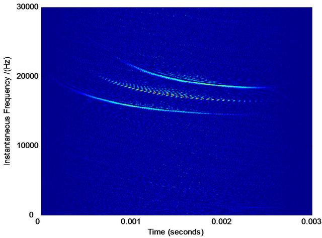
5.2. Experiments on Real-Life Data of Bat
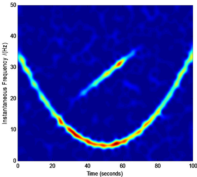
In this section, we will use the proposed method to ana-
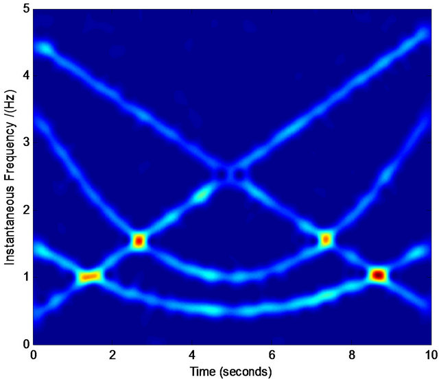
lyze the noised bat’s data (see Figure 9(a)). Since the data is disturbed by heavy noises, the true components in the data cannot be seen at all. Now we compared some methods with our proposed method to separate them. The compared methods include the empirical mode decomposition (EMD) [12] and the improved EMD (IEMD) [2]. IEMD cannot find the according assisted component and it fails to do this work because of the heavy noises (so there is no according result here). EMD can do this work, but its result (see Figure 9(f)) has no physical sense from the real-life nature. Instead, since our method makes full use of the fused time-frequency distribution and the function of soft-cutting in frequency domain, we finally obtain the two main decomposed components (see Figures 9(j) and (k)) with its rational physical interpretation (see Figure 9(i)).
6. Conclusions
AM-FM signals are widely used in various signal processing fields. When multiple AM-FM components are blended in noises, how to separate them is still a challenge. The tasks in the separation of multiple AM-FM components blended in noises are twofold: one is the denoising and another is the decomposition of these components. Especially when the frequency spectra of these components have overlapped regions in Fourier transform domain and even their instantaneous frequencies have crossed points in TFD, how to extract every AMFM component is nearly an open question to our knowledge. In this paper, we merge the two tasks (filtering the noises and decomposition of these components) to one new derived method.
Our contribution mainly includes the following. First, the Hilbert transform based decomposition is analyzed for the time-varying frequency components (i.e., nonstationary signals) via representative simulations and theoretical analysis. From these simulations and analysis we can obtain the conclusion: this method holds for the complicated case that the components have overlapped frequency regions in transform domain, which is a breakthrough in decomposing noised signals so that this demonstrates great potential valuable performance in the separation of components for more general/complicated cases. Second, based on the above analysis, a hypothesis with the condition that AM-FM components can be separated successfully based on Hilbert transform and assisted signal is proposed, which is supported by the experiments. After this, the time-varying bandpass filter (TVBF) based on assisted signals is proposed to separate the components blended in noises. The assisted signals used in TVBF are derived from the refined TFDs via image fusion and least squares optimization. The theoretical errors are also analyzed to bound the performance
 (a)
(a) (b)
(b)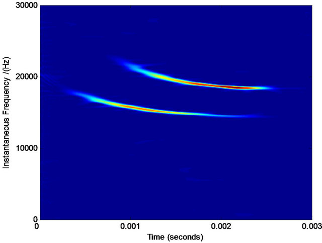 (c)
(c)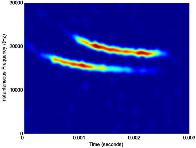 (d)
(d)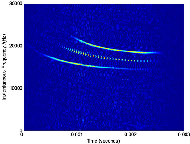 (e)
(e)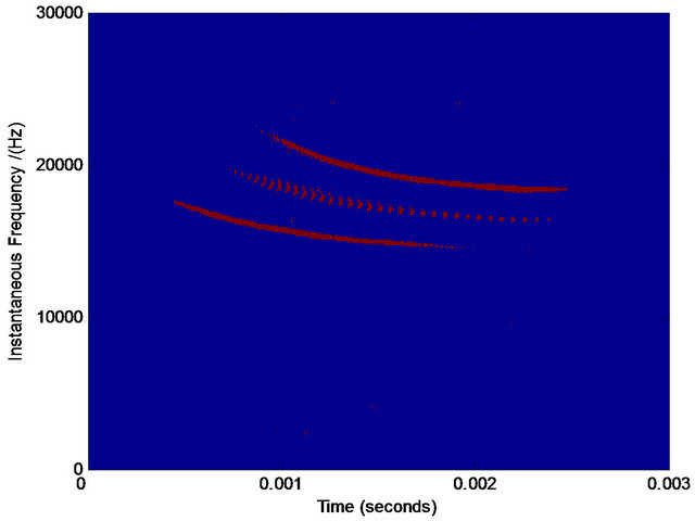 (f)
(f)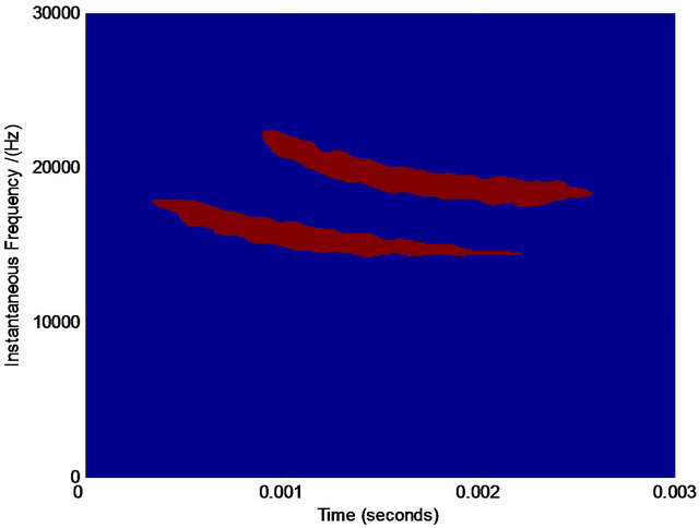 (g)
(g)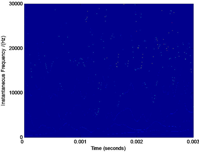 (h)
(h)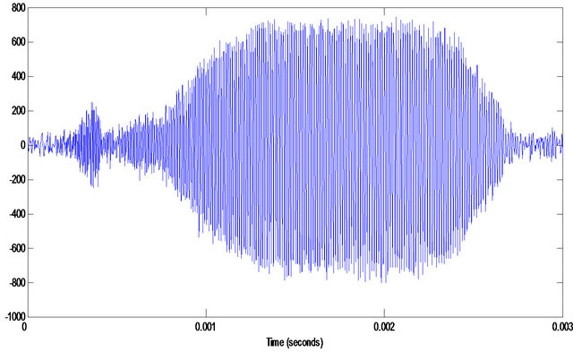 (i)
(i)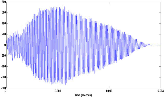 (j)
(j)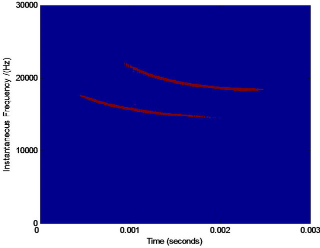 (k)
(k)
Figure 9. The analysis of real-life data of bat. (a) The noised real-life data of bat; (b) Wigner-Ville distribution; (c) pseudo Wigner-Ville distribution; (d) short Fourier transform distribution; (e) smoothed pseudo Wigner-Ville distribution; (f) HHT; (g) the fused result of (d) and (e); (h) the fused result of (b) and (c); (i) the fused result of (g) and (h); (j) the first component separated by our method; (k) the second component separated by our method.
of this method: the error is proportional to the product of the two parameters: ![]() and
and . Finally, some representative experiments on man-made and real-life data are shown to verify the efficiency of the proposed method and demonstrate the advantages over the other main methods.
Our biggest contribution of this paper is that we introduced a novel approach filtering and decomposing signals in a fully different manner. Our proposed TVBF seems like a “soft-cutter” and expediently cuts the components that have complicated instantaneous frequencies in frequency domain with rational physical sense. This method changes the idea of filtering and decomposing signals and will be a breakthrough from “soft” filtering and decomposing signals. In addition, one of our method’s biggest advantages is that we merge the two tasks (filtering and decomposing) to single one, which effecttively separate the components blended in noises that other methods fail to do.
REFERENCES
- X. D. Zhang, “Modern Signal Processing,” 2nd Edition, Tsinghua University Press, Beingjing, 2002.
- G. Xu, X. Wang and X. Xu, “Time-Varying FrequencyShifting Signal Assisted Empirical Mode Decomposition Method for AM-FM Signals,” Mechanical Systems and Signal Processing, Vol. 23, No. 8, 2009, pp. 2458-2469. doi:10.1016/j.ymssp.2009.06.006
- A. O. Boudraa and J. C. Cexus, “EMD-Based Signal Filtering,” IEEE Transactions on Instrumentation and Measurement, Vol. 56, No. 6, 2007, pp. 2196-2202. doi:10.1109/TIM.2007.907967
- J. G. Proakis and D. G. Manolakis, “Digital Signal Processing: Principles, Algorithms, and Applications,” 3rd Edition, Prentice-Hall, Englewood Cliffs, 1996.
- D. L. Donoho and I. M. Johnstone, “Ideal Spatial Adaptation via Wavelet Shrinkage,” Biometrica, Vol. 81, 1994, pp. 425-455. doi:10.1109/18.382009
- D. L. Donoho, “De-Noising by Soft-Thresholding,” IEEE Transactions on Information Theory, Vol. 41, No. 3, 1995, pp. 613-627.
- S. Mallat and Z. Zhang, “Matching Pursuits with TimeFrequency Dictionaries,” IEEE Transactions on Signal Processing, Vol. 41, No. 12, 1993, pp. 3397-3415. doi:10.1109/78.258082
- G. L. Xu, X. T. Wang, X. G. Xu and L. J. Zhou, “Improved EMD for the Analysis of FM Signals,” Mechanical Systems and Signal Processing, Vol. 33, No. 11, 2012, pp. 181-196. doi:10.1016/j.ymssp.2012.07.003
- F. Auger, P. Flandrin and P. Gonçalves, “Time-Frequency in Action with Matlab,” 2000. http://www.researchgate.net/publication/50207277_Time-frequency_in_action_with_Matlab
- B. Boashash, “Time-Frequency Signal Analysis and Processing—A Comprehensive Reference,” Elsevier Science, Oxford, 2003.
- L. Cohen, “Time-Frequency Analysis,” Prentice-Hall, New York, 1995.
- N. E. Huang, S. Zheng, R. L. Steven, et al., “The Empirical Mode Decomposition and the Hilbert Spectrum for Nonlinear Non-Stationary Time Series Analysis,” Proceedings of the Royal Society A, Vol. 454, 1998, pp. 903-995. doi:10.1098/rspa.1998.0193
- R. Deering and J. F. Kaiser, “The Use of a Masking Signal to Improve Empirical Mode Decomposition,” IEEE International Conference on Acoustics, Speech, and Signal Processing, Vol. 4, 2005, pp. IV485- IV488.
- N. Senroy, S. Suryanarayanan and P. F. Ribeiro, “An Improved Hilbert-Huang Method for Analysis of TimeVarying Waveforms in Power Quality,” IEEE Transactions on Power Systems, Vol. 22, No. 4, 2007, pp. 1843- 1850. doi:10.1109/TPWRS.2007.907542
- C. R. Gonzalez and E. R. Woods, “Digital Image Processing,” Pearson Education, 2nd Edition, Prentice Hall Press, Upper Saddle River, 2003.
- G. Chen and Z. Wang, “A Signal Decomposition Theorem with Hilbert Transform and Its Application to Narrowband Time Series with Closely Spaced Frequency Components,” Mechanical Systems and Signal Processing, Vol. 28, 2012, pp. 258-279. doi:10.1016/j.ymssp.2011.02.002
- R. Tao, B. Deng and Y. Wang, “Theory and Application of the Fractional Fourier Transform,” Tsinghua University Press, Beijing, 2009.
- G. Rilling and P. Flandrin, “One or Two Frequencies? The Empirical Mode Decomposition Answers,” IEEE Transactions on Signal Processing, Vol. 56, No. 1, 2008, pp. 85-95. doi:10.1109/TSP.2007.906771
- L. Angrisani, M. D’Arco, R. S. Lo Moriello, et al., “On the Use of the Warblet Transform for Instantaneous Frequency Estimation,” IEEE Transactions on Instrumentation and Measurement, Vol. 54, No. 4, 2005, pp. 1374- 1380. doi:10.1109/TIM.2005.851060
- J. P. Zhao and D. J. Huang, “Mirror Extending and Circular Spline Function for Empirical Mode Decomposition Method,” Journal of Zhejiang University Science, Vol. 2, No. 3, 2001, pp. 247-252. doi:10.1631/jzus.2001.0247
- Y. J. Deng, et al., “An Approach for Ends Issue in EMD Method and Hilbert Transform,” Chinese Science Bulletin, Vol. 46, No. 3, 2001, pp. 903-1005.
- J. Cheng, D. Yu and Y. Yang: “Discussion of the End Effects in Hilbert-Huang Transform,” Journal of Vibration and Shock, Vol. 24, No. 6, 2005, pp. 40-47.
- J. Wang, Y. Peng and X. Peng, “Similarity Searching Based Boundary Effect Processing Method for Empirical Mode Decomposition,” Electronics Letters, Vol. 43, No. 1, 2007, pp. 1-2.
- Y. Yang, W. M. Zhang, Z. K. Peng and G. Meng, “TimeFrequency Fusion Based on Polynomial Chirplet Transform for Non-Stationary Signals,” IEEE Transactions on Industrial Electronics, Vol. 60, No. 9, 2012, pp. 3948- 3956. doi:10.1109/TIE.2012.2206331
- E. Bedrosian, “A Product Theorem for Hilbert Transforms,” Memorandum RM-3439-PR, US Air Force Project RAND, 1962.
NOTES
*This work was fully supported by the NSFC (61002052) and partly supported by the NSFCs (61250006 and 60975016).