Agricultural Sciences
Vol.4 No.6A(2013), Article ID:33709,8 pages DOI:10.4236/as.2013.46A001
A recruitment forecasting model for the Pacific stock of the Japanese sardine (Sardinops melanostictus) that does not assume density-dependent effects
![]()
Department of Ocean Science and Technology, Tokyo University of Marine Science and Technology, Tokyo, Japan; sakurak@kaiyodai.ac.jp
Copyright © 2013 Kazumi Sakuramoto. This is an open access article distributed under the Creative Commons Attribution License, which permits unrestricted use, distribution, and reproduction in any medium, provided the original work is properly cited.
Received 20 April 2013; revised 20 May 2013; accepted 5 June 2013
Keywords: Stock-Recruitment Relationship; Sardine; Recruitment; Arctic Oscillation; Kuroshio Extension; Proportional Model; Forecasting
ABSTRACT
This study developed a recruitment forecasting model based on a new concept of the stock recruitment relationship. No density-dependent effect in the relationship was assumed in the model, which showed that fluctuations in recruitment and spawning stock biomass of Japanese sardine in the northwestern Pacific can be explained mainly by environmental factors and the effects of fishing. The February Arctic Oscillation (AO) and sea surface temperature over the southern area of the Kuroshio Extension (30 - 35˚N and 145 - 180˚E; KEST) were used as the environmental factors. The recruitment forecasting model is proposed:
 The values for recruitment (
 ), spawning stock biomass, (
 ), in year t, forecast by this model accurately reproduced those estimated by tuning virtual population analysis (VPA), and the pattern of variability in the stock recruitment relationship was also reproduced well. In conclusion, a density-dependent effect does not necessarily have to be included to explain the large variations in recruitment and the spawning stock biomass of the Japanese sardine.
1. INTRODUCTION
Among Japanese fisheries, the Japanese sardine (Sardinops melanostictus) is one of the most important species in the northwestern Pacific. In 1997 the Japanese Government introduced a total allowable catch (TAC) system for seven species including sardine. Sardine numbers began to increase during the 1960s and were very high in the 1980s, but decreased markedly in the early 1990s and have remained low. Since the TAC system was introduced, many fishermen who harvest sardine have opposed the schemes for management of the depleted populations. The government of Japan insists that a reduction in the TAC is necessary to rehabilitate the sardine population, but the fishermen insist that a reduction is not appropriate because the fluctuations in sardine population abundance are mainly caused by environmental factors.
To establish management schemes that are acceptable to fishermen but meet government management objectives, fisheries scientists need new models of sardine population abundance that can explain the extremely large fluctuations in recruitment and the spawning stock biomass.
Many studies have investigated the relationship between population fluctuations and environmental factors [1-4]. For instance, Noto [5], and Noto and Yasuda [6] studied the effect of environmental conditions, as represented by the sea surface temperature in the southern area of the Kuroshio Extension during winter. They raised the possibility that environmental factors determine annual changes in the survival of sardine, and also influence long-term fluctuations in the population and its distribution and migration patterns. Sunami [7] noted that water temperature and variations in the abundance of zooplankton (a sardine food source) influence the early growth stages of sardines (up to 1-year-old), which determines their survival rate.
Although most focus has been on the role of environmental factors, density-dependent effects are also believed to be important in explaining fluctuations in sardine stock abundance. For instance, Chen and Irvine [8] developed a stock-recruitment relationship model that incorporates environmental effects and performs better than the traditional Ricker model, on which it is based. Yatsu et al. [9] investigated the reproductive success of sardine with respect to water temperature, zooplankton density, intra-species competition, and density-dependent effects. Ishida et al. [10] adapted modified Ricker models that incorporate environmental factors, and proposed new stock-recruitment models for the Japanese sardine. However, all these models can be categorized as extended Ricker models because they stress the importance of density-dependent effects as well as environmental factors and fishing in the stock recruitment relationship.
Sakuramoto and Suzuki [11] showed even where there is no density-dependent effect in the stock-recruitment relationship, there is a high likelihood of detecting an apparent density-dependent effect on response to observed and/or process errors; the latter is considered to occur mainly because of environmental changes. They also criticized the a priori assumption of a density-dependent effect on the sardine stock recruitment relationship, because such an assumption can lead to an underestimate of the effects of environmental factors. They concluded that when we analyze the stock recruitment relationship data of the northwestern Pacific sardine stock, no density-dependent effect can be detected, and a proportional model should be used for assessment of the stock recruitment relationship for Japanese sardine.
The purpose of this study was to present a recruitment forecasting model based on a stock recruitment relationship where no density-dependent effect is assumed, and to show that large fluctuations in recruitment and the spawning stock biomass of sardine can be explained only by environmental factors and the effects of fishing.
2. MATERIAL AND METHODS
2.1. Data
The catch number, average weight, maturity rate, and the natural mortality coefficient were recorded by age and year for the northwestern Pacific sardine stock from 1976 to 2012 [12]. The number of fish and the fishing mortality coefficients by age in each year were also used from the report. [12]. Data on the Arctic Oscillation (AO) for February was obtained from the NOAA Climate Prediction Center [13], and the sea surface temperature over the southern area of the Kuroshio Extension for 30 - 35˚N and 145 - 180˚E (KEST) in February was obtained from Ishii [14].
2.2. Recruitment Forecasting Model
The recruitment forecasting models developed comprised two parts: one concerning the role of the stock recruitment relationship f(S), and the other the role of environmental factors, g(*), as shown in Equation (1):
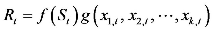 (1)
(1)
where Rt is the recruitment at the beginning of fishing period in year t, St is the spawning stock biomass at the beginning of the fishing period in year t, and x1,t, , xk,t are variables related to the environmental factors in year t. Parameter k denotes the number of variable that are related to the environmental factors.
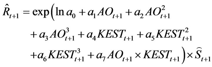
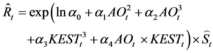
Based on the method of Sakuramoto et al. [15], a proportional model was assumed for the stock recruitment relationship; thus, no density dependent effect was incorporated in the model. For simplicity only two environmental factors, AO and KEST in February (AOt and KESTt, respectively), were included in the model, as described by Equation (2): ![]()
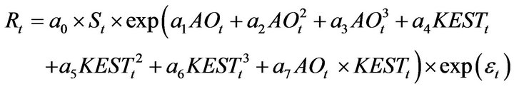 (2)
(2)
where, 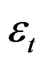 is an error term having a log normal distribution with mean 0 and variance
 .
.
The parameters were estimated by regression analysis using Equation (3), and the statistically significant partial regression coefficients were chosen.
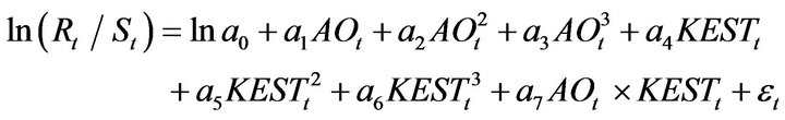 (3)
(3)
2.3. Simulation Process
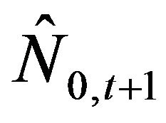
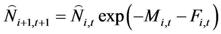
Simulations were conducted as follows. Initial values were assigned for the population number from age 0 to 5+ (5 years old and older) in 1976 (N0,76, N1,76, N2,76, N3,76, N4,76, and N5+,76 [12]. N0,76 indicates the recruitment number in 1976 (R76).
The recruitment number at the beginning of the fishing period in the following year, 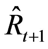 =
= , was calculated using Equation (4):
 (4)
(4)
The number of fish from age 1 to 4 in the following year, 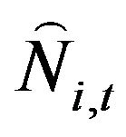 , was calculated using Equation (5), when t = 1976, the initial values, Ni,t, (i = 1, 2,
  , 5+) are used.
 (5)
(5)
The number of fish at age 5 and older in the following year (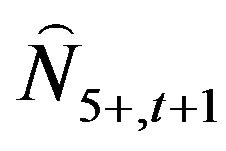 ) was calculated using Equation (6):
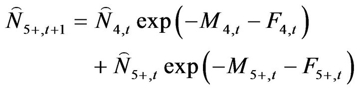 (6)
(6)
where Mi,t, and Fi,t are the natural mortality coefficient at age i in year t and the fishing mortality coefficient at age i in year t, respectively.
The spawning stock biomass in the following year (t + 1) was calculated using Equation (7):
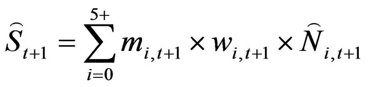 (7)
(7)
where mi,t+1 and wi,t+1 are the maturity rate at age i in year t + 1 and the mean weight at age i in year t + 1, respectively. This process was repeated until t + 1 = 2012.
The partial regression coefficients estimated by the least square method for Equation (3) were slightly modified to minimize the sum of square value (SS) defined by Equation (8):
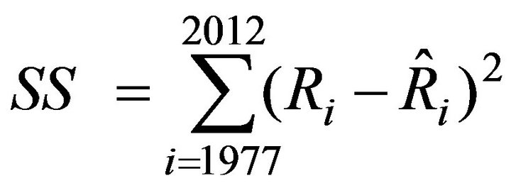 (8)
(8)
where  and
and  are the referred [12] and forecast recruitment, respectively.
2.4. Forecasting the Recruitment in 2013
When the values for the AO and the KEST for February 2013 are available it will be possible to predict the recruitment in 2013 using the forecasting model proposed here, provided that the maturity rate by age and the mean weight by age in the year 2013 are the same as in 2012. The recruitment in 2013 can be calculated by VPA after the middle of the following year 2014, when the catch at age data, maturity rate, and mean weight by age for 2013 will have been compiled. Therefore, the recruitment in 2013 can forecast more than one year earlier by using this model.
3. RESULTS
3.1. Parameters Estimated by Regression Analysis
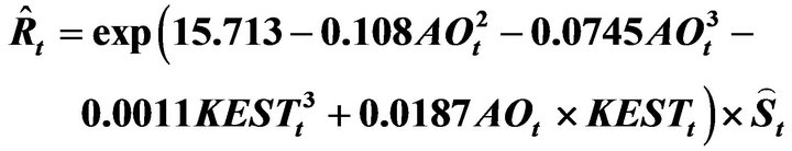
A recruitment forecasting model was chosen for which all the partial regression coefficients were statistically significant. The parameters and the statistically significant probabilities are shown in Table 1. The resulting model is shown in Equation (9):
 (9)
(9)
The partial regression parameters were then modified to reduce the SS value calculated by Equation (8). More The
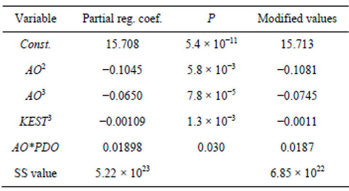
Table 1. Estimated partial regression coefficeints and modified parameters used in the simulations.
suitable parameters were sought within the ranges [ai − hi, ai + hi], where ai is the partial regression parameters estimated using the least squares method and hi denotes the interval given for each parameter. The modified partial regression coefficients are also shown in Table 1. The SS value was reduced from 5.22 ´ 1023 to 6.85 ´ 1022 using this approach.
3.2. Results of Forecasts
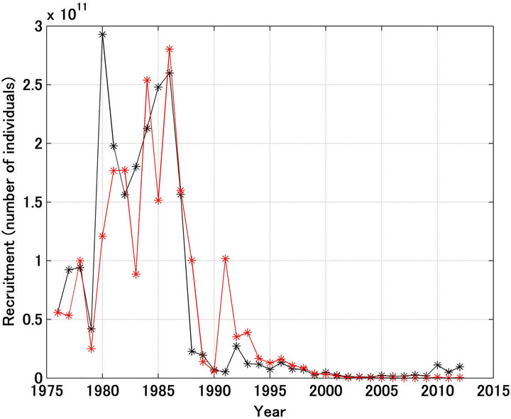
Figure 1(a) shows the referred recruitment [12] and that forecast using the model. While large differences were found for 1980, 1983, 1985, 1988, and 1991, generally the pattern of the variation was reproduced well. In particular, the dramatic decline in recruitment from 1986 to 1989 was reproduced well, regardless of the assumption of a density-dependent effect in the stock recruitment relationship. Figure 1(b) shows the case where the scale in the Y-axis was enlarged after 1995. The referred recruitment decreased until 2004, after 2005 there was an apparent slight increase, and since 2010 the level of recruitment has been remarkably high. The forecast pattern was quite different, with recruitment continuing to decrease after 2004. The reasons for these differences are discussed below.
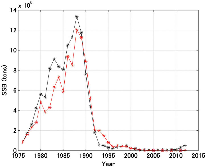
Figure 2(a) shows the spawning stock biomass calculated using Equation (7). Prior to 1988 the forecast spawning stock biomass was lower than the referred biomass. This is because prior to 1988 the forecast recruitment was less than the referred recruitment, except in 1983 and 1984. However, the increasing tendency referred was reproduced well. On the contrary, after 1989 the decreasing tendency referred was reproduced significantly well except in 1993 and 1994.
Figure 2(b) shows the case where the scale in the Y-axis was enlarged after 1995. The referred spawning stock biomass decreased until 2005, was stable until 2008, and subsequently increased markedly. The forecast pattern was substantially different, with the spawning stock biomass continuing to decrease after 2005, following the same pattern as recruitment. The reasons for these
 (a)
(a)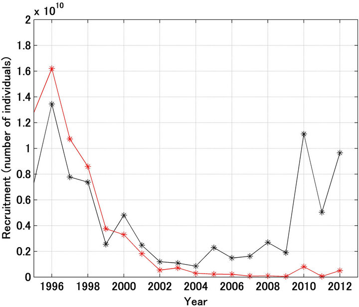 (b)
(b)
Figure 1. Trajectories in recruitment forecasted and referred of Japanese sardine (a); Trajectories shown in enlarged scale (b). Black and red lines indicate the referred and forecasted recruitment, respectively.
differences are also discussed below.
Figure 3 shows the forecast and referred stock recruitment relationships. The variables on both the x and y axes were estimated, and some of the forecast and referred data points do not coincide well. However, the trajectory showing a loop rotating clockwise was reproduced well.
Figure 4 shows the forecast and referred recruitment per spawning stock biomass (RPS) [12]. The fluctuations in RPS were large, but the trends were reproduced well except for the years 1977, 1980, 1982, 1991, 2005, and 2008. In 2010 the forecast value estimated by this model was extremely large relative to the referred one.
3.3. Validity of the F Estimates after 2001
This section considers the validity of the value of the
 (a)
(a)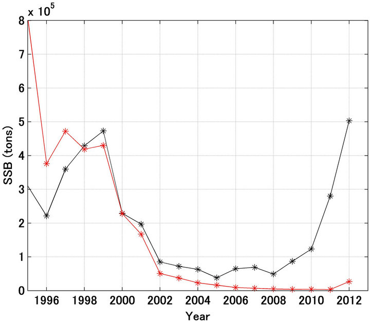 (b)
(b)
Figure 2. Trajectories in spawning stock biomass forecasted and referred of Japanese sardine (a); Trajectories shown in enlarged scale (b). Black and red lines indicate the referred and forecasted spawning stock biomass, respectively.
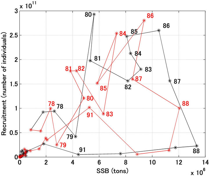
Figure 3. Stock-recruitment relationship for Japanese sardine in the northwestern Pacific from 1976 to 2012. Black and red indicate the referred and forecasted relationship, respectively. Figures denote the year.
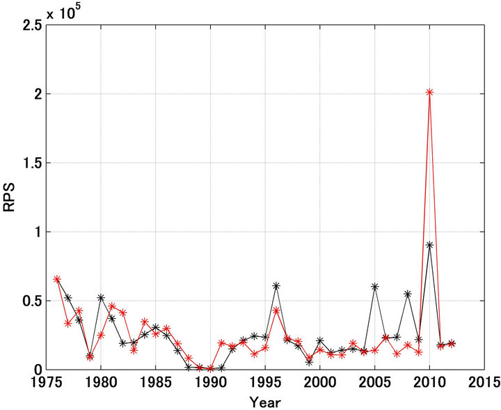
Figure 4. Recruitment per spawning stock biomass (RPS) for Japanese sardine in the northwestern Pacific from 1976 to 2012. Black and red indicate the referred and forecasted RPS, respectively.
fishing mortality coefficient, Fa,t. The results shown in Figures 1(b) and 2(b) indicate that the forecast and referred values and trends were significantly different. Figure 5 shows the referred and forecast catch trajectories by age. For ages 0 after 2000, the forecast catches were extremely low relative to the referred catches, and the forecast recruitment and spawning stock biomass after 2005 were much less than the referred values (Figures 1(b) and 2(b)). This reduction in the recruitment and spawning stock biomass may not have been a consequence of overfishing. Because the forecasted catches in ages 0 and 1 were low after 2000. Figure 6 shows the fishing mortality coefficient trajectories by age [12]. Figure 6 shows that after 2001 the fishing mortality coefficients for ages 0 and 1 were extremely large compared with those in the previous years.
One explanation for the extremely low level of recruitment and spawning stock biomass after 2005 is that the values were erroneously forecast in response to the large fishing mortality coefficients used in the simulation. Thus, when the sardine population was extremely low the fishermen tended to target species for which the biomass was greater (in this case mackerel or Japanese anchovy). The VPA method did not incorporate qualitative changes in fishing effort in estimating the fishing mortality coefficient. Therefore, it is highly likely that the fishing mortality coefficient was overestimated during the period when the population abundance was extremely low.
Figure 1(b) indicates a large difference between forecasted and referred recruitment trends since 2005. The spawning stock biomass was based on mature sardine (1 - 5 years old). Therefore, the spawning stock biomass in 2005 was determined based on sardines of age 1 in 2001,
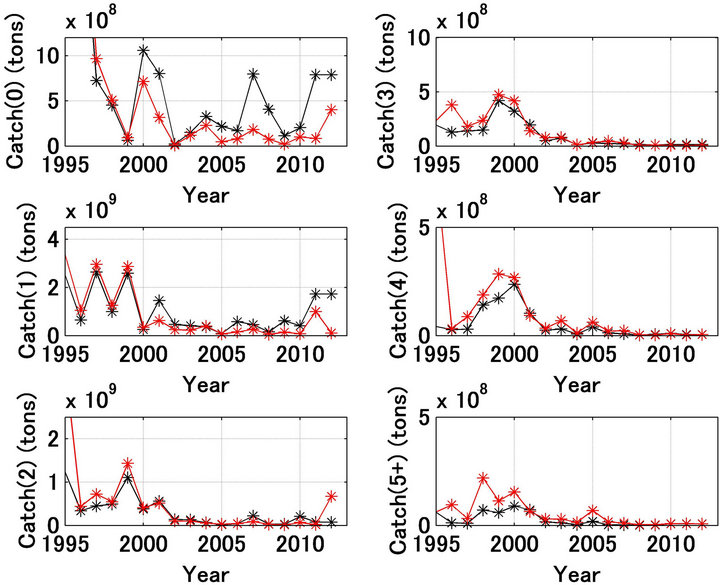
Figure 5. Trajectories of catch by age for Japanese sardine in the northwestern Pacific. Black and red indicate the referred and forecasted, respectively.
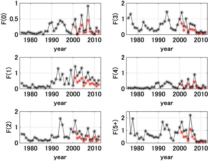
Figure 6. Trajectories of fishing mortality coefficients by age for Japanese sardine in the northwestern Pacific. Black and red are the values referred and the half of the referred values from 2001, respectively.
and up to age 1 in 2005. If the fishing mortality coefficient after 2001 was much lower, the spawning stock biomass would increase, and thus the recruitment would also be expected to increase.
Simulations were conducted when the smaller fishing mortality coefficient, 100d% of fishing mortality coefficient was used. The parameter d was determined so as to make the sum of square value (SS2) the smallest, which is defined by Equation (10).
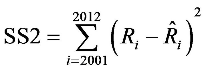 (10)
(10)
SS2 was smallest when d was set at 0.50. In Figure 6, it was also shown that the fishing mortality coefficient after 2001 was half of that referred. Figures 7-9 show
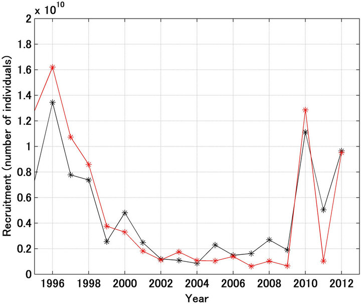
Figure 7. Trajectories in recruitment forecasted (red line) and referred (black line) when the fishing mortality coefficient by age after 2001 was set at half of the referred values.
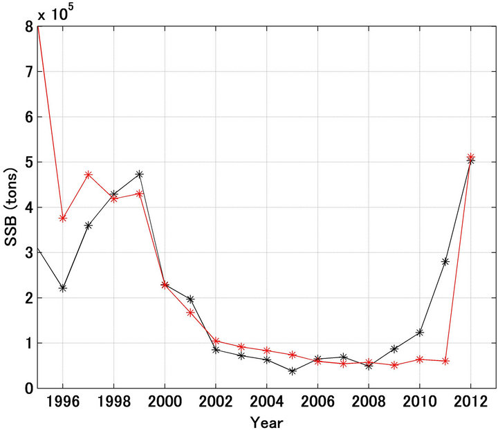
Figure 8. Trajectories in spawning stock biomass forecasted (red line) and referred (black line) when the fishing mortality coefficient by age after 2001 was set at half of the referred values.
the forecast recruitment, spawning stock biomass, and stock recruitment relationship (respectively) when d was set at 0.50. The forecast values were markedly improved using this approach.
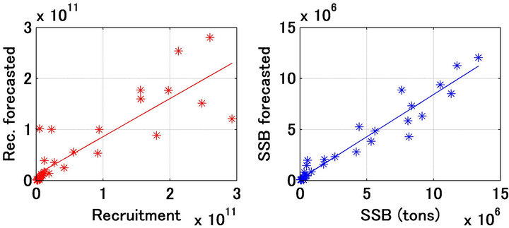
Figures 10(a) and (b) show a comparison of the forecast and referred recruitment and spawning stock biomass. The determination coefficients were 0.755 and 0.942, respectively.
3.4. Forecasting the Recruitment in 2013
When values of the AO and the KEST for February 2013 are available it will be possible to forecast the re-
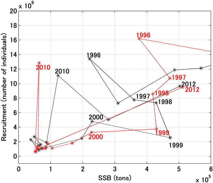
Figure 9. Stock-recruitment relationship for Japanese sardine in the northwestern Pacific from 1996 to 2012. Black and red lines indicate the referred and forecasted when the fishing mortality coefficient by age after 2001 were set at half of the referred values. Figure denotes the year.
 (a) (b)
Figure 10. Relationship between recruitment (number of individuals) forecasted and referred (a); Relationship between spawning stock biomass (tons) forecasted and referred (b).
cruitment in 2013 using the forecasting model proposed here, provided that the maturity rate by age and mean weight by age for 2013 are the same as in 2012. The recruitment in 2013 was forecast to be 61.3 ´ 108, which is 35.6% less than in 2012. Corresponding to this value, the spawning stock biomass in 2013 was estimated at 346,000 tons, which is 32.3% less than in 2012. However, the former will vary depending on the maturity rate and mean weight by age in 2013. Although these are estimated values it is important to estimate values that can be confirmed in the following year, as this can aid assessment of the validity of the forecasting model, and provide important information for fisheries resource managers.
4. DISCUSSION
A noteworthy finding of the present study was that large fluctuations in recruitment and the spawning stock biomass were reproduced remarkably well by the proposed model, which did not assume a density-dependent effect on the stock recruitment relationship. As shown in Figure 3, a large loop emerged in the stock recruitment relationship for the northwestern Japanese sardine stock; however, it is difficult to explain how the loop emerged. Although, this loop is never produced with density-dependent effects, the recruitment forecasting model proposed in this study can reproduce a similar loop in the stock-recruitment relationship in response to the fluctuations of environmental factors.
Shimoyama [16] forecasted the recruitment and spawning stock biomass using the models,  . As the
 , she used not only a proportional model but also the models that had the density-dependent effects, and showed the similar results regardless of what kinds of the stock-recruitment models assumed. However, she only used the two independent variables, AOt and KESTt in the function g(AOt, KESTt). Therefore, the forecasting did not reproduce the recruitment well. Especially the steep decline from 1986 to 1989 could not reproduce well. In this model, the performance was improved much better than the results of Shimoyama [16].
In this study, I did not compare the models between the cases when density-dependent effects were assumed or not. Because, if the results for the case when the density-dependent effects were assumed was little better than the case when they did not assume, as Sakuramoto and Suzuki [11] showed that it did not necessarily indicate the validity of density-dependent models. It just indicated that other environmental factors that would control the recruitments should be incorporated.
Sakuramoto [17] showed that the clockwise loop shown in the stock-recruitment relationship of the Japanese sardine could be explained by the mechanism, which constructed two assumptions. One is the recruitment is proportional to the spawning stock biomass and another is the spawning stock biomass fluctuates cyclically in response to environmental fluctuations. The simulation shown in this study supported the validity of the assumptions. That is, essentially the recruitment is proportional to the spawning stock biomass, however, the recruitments were changed in response to environmental fluctuations, and the spawning stock biomass fluctuates cyclically, and then the clockwise loop emerged, which is never explained by the density-dependent effect on the stock-recruitment relationship.
Shimoyama et al. [18], Sakuramoto et al. [15], and Sakuramoto and Suzuki [11] noted that no density dependent effect could be detected in data related to the stock recruitment relationship for the Japanese sardine, and suggested that a proportional model be used to describe the stock recruitment relationship for this species. However, the criticism always noted for this conclusion is that in this case the population will increase infinitely or deplete to zero when the environmental conditions are constant. Therefore, assuming a proportional model for the stock recruitment relationship of Japanese sardine appears inappropriate. However, this criticism is not logical because environmental conditions never remain constant in the real world. Therefore, even if an unrealistic conclusion is derived from an unrealistic assumption (e.g., that environmental conditions are constant), this does not imply that a proportional model is inappropriate. As shown in this study, as environmental conditions fluctuate the population never increased infinitely or depleted to zero, even when the stock recruitment relationship was expressed using a proportional model.
Data for the Pacific decadal oscillation index (PDO) were also used as an environmental condition, but in this model the partial regression coefficients related to the PDO were not statistically significant. In future, if other environmental conditions are found that explain the fluctuations in recruitment more accurately, the forecasting model can be further improved.
The sensitivity tests for the F values after 2001 indicated that there was a possibility that F values were overestimated when the population abundance is extremely low. The actual F values may be almost the half of those of estimated [12]. The sensitivity tests also indicated that fishing is an important factor controlling the population trajectories, especially when the population biomass is low and environmental conditions are unfavorable for the sardine population.
The earthquake and tsunami after the earthquake occurred on March 11, 2011 must have changed extremely the environmental conditions along the Pacific coast of Japan. These changes might affect the survival of the fish recruited after 2012. The forecasting is done using only two environmental factors, AO and KEST in February, therefore, if other environmental conditions, which affect the recruitment, have extremely changed, of course, the performance of the forecasting will not be well.5. ACKNOWLEDGEMENTS
I thank Japan Meteorological Agency, for providing the water temperature data for the Kuroshio extension area.
REFERENCES
- Ebisawa, Y. and Kinoshita, T. (1998) Relationship of surface water temperature in Boso-Sanriku Area Sea and recruitment per spawning biomass of the Japanese sardine. Report of Ibaragi Prefecture Fisheries Experimental Station, 36, 49-55.
- Kuroda, K. (1991) Studies on the recruitment process focusing on the early life history of the Japanese sardine Sardinops melanostictus (SCHLEGEL). Bulletin of the National Research Institute of Fisheries Science, 3, 25- 278.
- Sugisaki, H., Matsuo, Y., Yokouchi, K. and Takahashi, Y. (1994) Distribution of larvae and juveniles of Japanese sardine, Sardinops melanostictus, off the east coast of Honshu Island, Japan. Bulletin of the Japanese Society of Fisheries Oceanography, 58, 336-338.
- Tomosada, A. (1988) Long-term variations in water temperature and sardine catch. Bulletin of the National Research Institute of Fisheries Science, 126, 1-9.
- Noto, M. (2003) Population decline of the Japanese sardine in relation to sea surface temperature in the Kuroshio Extension. Marine Science Monthly, 35, 32-38.
- Noto, M. and Yasuda, I. (1999) Population decline of the Japanese sardine with relation to the sea-surface temperature in the Kuroshio Extension. Canadian Journal of Fisheries and Aquatic Sciences, 56, 973-983.
- Sunami, Y. (1993) Modeling of the variability in stock abundance of Japanese sardine from a viewpoint of its food density. Journal of the Shimonoseki University of Fisheries, 41, 1-8.
- Chen, D.G. and Irvine, J.R. (2001) A semi-parametric model to examine stock-recruitment relationships incorporating environmental data. Canadian Journal of Fisheries and Aquatic Sciences, 58, 1178-1186.
- Yatsu, A., Watanabe, T., Ishida, M. Sugisaki, H. and Jacobson, L.D. (2005) Environmental effects on recruitment and productivity of Japanese sardine Sardinops melanostictus and chub mackerel Scomber japonicus with recommendations for management. Fisheries Oceanography, 14, 263-278. doi:10.1111/j.1365-2419.2005.00335.x
- Ishida, Y., Funamoto, T., Yabuki, K., Honda, S., Nishida, H. and Watanabe, C. (2009) Management of declining Japanese sardine, chub mackerel and walleye pollock fisheries in Japan. Fisheries Research, 100, 68-77. doi:10.1016/j.fishres.2009.03.005
- Sakuramoto, K. and Suzuki, N. (2012) Effects of process and/or observation errors on the stock-recruitment curve and the validity of the proportional model as a stock-recruitment relationship. Fisheries Science, 78, 41-54. doi:10.1007/s12562-011-0438-4
- Kawabata, A., Honda, S., Watanabe, C. and Kubota, H. (2013) Stock assessment and evaluation for the Pacific stock of Japanese sardine (fiscal year 2012). In: Marine Stock Fisheries Stock Assessment and Evaluation for Japanese Waters (Fiscal Year 2012), Fisheries Agency and Fisheries Research Agency of Japan, 15-44.
- Arctic Oscillation, NOAA Climate Prediction Center. http://www.cpc.ncep.noaa.gov/products/precip/CWlink/daily_ao_index/monthly.ao.index.b50.current.ascii.table
- Ishii, M., Shouji, A., Sugimoto, S. and Matsumoto, T. (2005) Objective analyses of sea-surface temperature and marine meteorological variables for the 20th century using ICOADS and the Kobe collection. International Journal of Climatology, 25, 865-879. doi:10.1002/joc.1169
- Sakuramoto, K., Shimoyama, S. and Suzuki, N. (2010) Relationship between environmental conditions and fluctuations in the recruitment of Japanese sardine, Sardinops melanostictus, in the northwestern Pacific. Bulletin of the Japanese Society of Fisheries Oceanography, 74, 88-97.
- Shimoyama, S. (2006) A study on the fluctuations in recruitment for Japanese sardine Sardinops melanostictus in the North-Western Pacific and ocean environmental factors. Master Thesis, Tokyo University of Marine Science and Technology, Tokyo.
- Sakuramoto, K. (2005) Does the Ricker or Beverton and Holt type of stock-recruitment relationship truly exist? Fisheries Science, 71, 577-592. doi:10.1111/j.1444-2906.2005.01002.x
- Shimoyama, S., Sakuramoto, K. and Suzuki, N. (2007) Proposal for stock-recruitment relationship for Japanese sardine Sardinops melanostictus in the North-western Pacific. Fisheries Science, 73, 1035-1041. doi:10.1111/j.1444-2906.2007.01433.x