Advances in Aerospace Science and Technology
Vol.04 No.01(2019), Article ID:90889,15 pages
10.4236/aast.2019.41001
A Data-Driven Adaptive Method for Attitude Control of Fixed-Wing Unmanned Aerial Vehicles
Meili Chen, Yuan Wang
Key Laboratory of Fundamental Science for National Defense-Advanced Design Technology of Flight Vehicle, Nanjing University of Aeronautics and Astronautics, Nanjing, China

Copyright © 2019 by author(s) and Scientific Research Publishing Inc.
This work is licensed under the Creative Commons Attribution International License (CC BY 4.0).
http://creativecommons.org/licenses/by/4.0/


Received: January 4, 2019; Accepted: February 27, 2019; Published: March 1, 2019
ABSTRACT
In this paper, a real-time online data-driven adaptive method is developed to deal with uncertainties such as high nonlinearity, strong coupling, parameter perturbation and external disturbances in attitude control of fixed-wing unmanned aerial vehicles (UAVs). Firstly, a model-free adaptive control (MFAC) method requiring only input/output (I/O) data and no model information is adopted for control scheme design of angular velocity subsystem which contains all model information and up-mentioned uncertainties. Secondly, the internal model control (IMC) method featured with less tuning parameters and convenient tuning process is adopted for control scheme design of the certain Euler angle subsystem. Simulation results show that, the method developed is obviously superior to the cascade PID (CPID) method and the nonlinear dynamic inversion (NDI) method.
Keywords:
Data-Driven, Adaptive Method, Attitude Control, Unmanned Aerial Vehicles (UAV), Internal Model Control

1. Introduction
The performance of the attitude controller of a fixed-wing UAV determines the quality of its autonomous flight. Some accurate mathematical model-based methods were proposed for the attitude control, for example, PID and LQR methods (linearized model based) [1] [2] [3] , adaptive control method [4] , feedback linearization method [5] [6] and nonlinear dynamic inversion method [7] [8] . For some other methods, perturbation within a small range is allowed [9] [10] or accurate mathematical model is not a necessity [11] [12] .
Though these methods have achieved their purpose, there are still some drawbacks. Firstly, as the UAV system is strongly coupled, highly nonlinear and time variant, etc., approximated models cannot fully represent all characteristics of plant model. In the meantime, accurate model is hard to obtain, too costly or even inapplicable; secondly, designing controller is complex and tuning is tedious due to too many parameters.
A data-driven control method for designing attitude control law of fixed-wing UAV is thus developed. The control system is divided into two cascade subsystems, including an inner loop system for angular velocity control and an outer loop system for Euler angle control. As the angular velocity control system contains all model information (certainties and uncertainties), a novel data-driven MFAC [13] [14] method is adopted for the inner loop angular velocity control law design. MFAC has been wildly used in some fields [15] [16] , but hardly in aeronautic field. As we know of, only one paper [17] studied the application of MFAC to design control law for tracking horizontal trajectory of fixed-wing UAV, but it took no consideration of attitude control, which is an unneglectable problem. The method developed in our paper uses no model information, but only I/O data of UAV to obtain control law by optimizing the deflection angles of control surfaces in real-time. The model of outer loop control system, which is universal and contains no uncertainty, depicts the kinematic relationship between Euler angel and angular velocity. Thus the IMC method, which was hardly used in fixed-wing UAV application but widely in other fields [18] [19] [20] , is used to design outer loop Euler angle control law. IMC based controller is featured with less tuning parameters and simple tuning process, for example, only one parameter needs to be tuned for each channel of the roll, pitch, and yaw Euler angles.
2. Theory of the Model Free Adaptive Control
2.1. Full Formation Dynamic Linearization Method
Consider the following general single-input-single-output (SISO) nonlinear system:
(1)
which satisfies the following two assumptions:
A1: Function is smooth; and its continuous and bounded partial derivatives and exists;
A2: The system satisfies generalized Lipschitz condition, that is, for two real numbers , and a positive number b, the system satisfies:
(2)
In above, and represent input and output of the system, respectively. and are two integers. is a nonlinear mapping.
Denote
(3)
and
(4)
where, and are integers called pseudo order (PO).
Theorem [13] : For the nonlinear system mentioned above that satisfies the A1 and A2, at a given condition of and , when , there must be a time-varying vector called pseudo gradient (PG) , which can transform the system into the following FFDL model:
(5)
and for an arbitrary time k, is bounded.
Proof: See [13] .
2.2. Control Law Design
Denote as reference signal. The cost function of input signal is selected as:
(6)
where, is a weighting factor.
According to Equations (5) and (6) and let , the control law can be derived as:
(7)
where, , .
In Equation (7), only PG is unknown and needs to be updated online.
To obtain PG, the following cost function is adopted:
(8)
where, is a weighting factor.
Letting yields
(9)
where, .
The reset conditions for PG are:
, if or or
(10)
where, is a small positive number.
3. Model for Unmanned Aerial Vehicles
The model described here is only used to generate flight data for simulations. The nonlinear model of a UAV [21] used in the research as a studying case is listed as follows.
Rotational equations:
(11)
(12)
In which , and are virtual inputs which are used in the following of the design of Euler angle control law. And
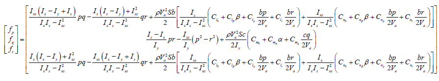 (13)
(13)
(14)
Translational equations:
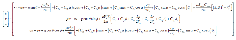 (15)
(15)
and
(16)
In the above equations, m and g represent mass and gravitational constant, respectively; , , , and represent moments of inertia; , , and represent roll, pitch, and yaw angle, respectively; p, q, and r represent roll, pitch, and yaw angular velocity, respectively; , , and are deflection angles of aileron, elevator, and rudder, respectively; is throttle, ranging from 0 to 1; b represents wing span; c represents chord length; S represents wing area; represents air speed; represents air density; and are attack and sideslip angle, respectively; and are coefficients with respect to propeller. , , , , , and are aerodynamic derivatives with respect to roll moment; , , , and are aerodynamic derivatives with respect to pitch moment; , , , , , and are aerodynamic derivatives with respect to yaw moment; , , , and are aerodynamic derivatives with respect to lift; , , , , , and are aerodynamic derivatives with respect to side force; , , , and are aerodynamic derivatives with respect to drag. Appendix E of Reference [21] also gives specific values of the above symbols.
4. Brief Introduction of Internal Model Control
The general structure of an IMC-based control system [18] is depicted in Figure 1; where, is called internal model. represents the plant, represents reference signal, represents the output signal, represents input signal of the plant, is disturbances and is the internal model controller. is the internal model controller that has an expression like
(17)
where, includes the parts with minimum phase of . is a low pass filter that has a formation like
(18)

Figure 1. The general structure of internal model control.
is called filter coefficient. Rationality of can be guaranteed by selecting appropriate value of n.
Thus, the two transfer functions of the above system can be obtained as:
(19)
(20)
Hence, if and satisfy the following two conditions:
(21)
(22)
Equations (19) and (20) turn into:
(23)
(24)
Therefore, building on conditions (23) and (24), the system can track the reference signal and at the same time, would theoretically not be influenced by disturbances.
5. Control Scheme
In this part, the attitude control laws are derived. In controlling a fixed-wing UAV, usually, deflecting aileron generates roll movement, deflecting elevator generates pitch movement, and deflecting rudder generates yaw movement. The overall control scheme is shown as:
Applying Equations ((7), (9), and (10)) yields the control laws of roll, pitch, and yaw angular rates, shown as:
Roll rate:
(25)
, if or or
(26)
(27)
Pitch rate:
(28)
, if or or
(29)
(30)
Yaw rate:
(31)
, if or or
(32)
(33)
The Euler angle control laws are included in Equation (11) and Figure 2.
6. Numerical Validation
Simulation was carried out in the MATLAB environment by writing .m file to demonstrate the feasibility and superiority of the method developed by making
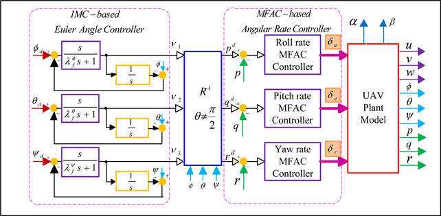
Figure 2. Illustration of the overall control scheme.
comparison with CPID and NDI methods. In the simulation, the UAV was under external disturbances.
6.1. Value of Variables and Parameters
Parameter values of algorithms are shown as (Table 1):
Reference signals:
(34)
6.2. Numerical Validation
In this part, the control simulation of the small UAV was performed with the UAV under external low frequency disturbances. Simulation results are as follows:
From the figures the following conclusions can be drawn:
Figures 3-5 reveal that, without using any model information of the UAV, the developed data-driven method is obviously superior to the CPID method (also a data-driven method) and the NDI method (requires detailed model information) in control performance. The fundamental reason is that the method develop has a better control performance on body rate control, namely, realizing a better performance in dealing with uncertainties, which is revealed in Figures 6-11.
The essential difference between the MFAC method and the CPID method is the acquisition of dynamic model, see Equations (9) and (10). In the MFAC method, because of the identification of PG, a dynamic model can be obtained, which is foundation for optimal control law design, making deflection angles of control surfaces at each time point are optimum. This is also why the varying frequency of the control surfaces of the method developed is so high in Figures 6-8. The optimum control laws take into account of all uncertainties, thus even they may disturb the system, these control laws will make the output of UAV system track and approximate reference signal (see Figures 9-11). While for the

Table 1. Parameters of the control scheme.

Figure 3. Roll angle response.

Figure 4. Pitch angle response.

Figure 5. Yaw angle response.

Figure 6. Deflection angle of aileron.

Figure 7. Deflection angle of elevator.

Figure 8. Deflection angle of rudder.

Figure 9. Angular rate of data-driven method.

Figure 10. Angular rate of CPID method.

Figure 11. Angular rate of NDI method.
most widely used CPID-based controller that lacks dynamic model obtaining capabilities, its deflection angles at each sampling point are not optimum and thus cannot cover the whole flight envelop with best performance (the control law may be optimal in a certain short time range, see 0 - 2.3 seconds in first and third enlarged figures in Figure 10, but not in the whole range). As for the NDI method, it relies on accurate model information and some of them such as the external disturbances are hard to be obtained, resulting in poor robustness of this method. Besides, the deflection angles by NDI are not necessarily optimum at each sampling point under unmodeled uncertainties.
7. Conclusion
The attitude control of fixed wing UAVs is studied based on the characteristics of inner loop and outer loop control systems, and realized by using MFAC to design the control law of inner loop angular velocity system and IMC to design that of Euler angle system. Firstly, the MFAC based controller has achieved inner loop angular velocity control using only I/O data without any model information. The IMC based controller has realized outer loop Euler angle control using a few tuning parameters (only one for each channel) and easy tuning process. Secondly, compared with conventional model-free CPID method and detailed model-based NDI method, it is discovered that the method developed is capable of dealing with strong coupling and highly nonlinear system such as that of fixed-wing UAVs; and it shows superiority in dealing with disturbances.
Acknowledgements
This publication was supported by the Priority Academic Program Development of Jiangsu Higher Education Institutions and the Advanced Research Project of Army Equipment Development (No.301020803).
Conflicts of Interest
The authors declare no conflicts of interest regarding the publication of this paper.
Cite this paper
Chen, M.L. and Wang, Y. (2019) A Data-Driven Adaptive Method for Attitude Control of Fixed-Wing Unmanned Aerial Vehicles. Advances in Aerospace Science and Technology, 4, 1-15. https://doi.org/10.4236/aast.2019.41001
References
- 1. Bagheri S., Jafarov T., Freidovich L. and Sepehri, N. (2016) Beneficially Combining LQR and PID to Control Longitudinal Dynamics of a SmartFly UAV. Proceedings of the 7th Annual IEMCON, Vancouver, 13-15 October 2016, 1-6. https://doi.org/10.1109/IEMCON.2016.7746309
- 2. Peng, Z. and Liu, J.K. (2011) On New UAV Flight Control System Based on Kalman & PID. Proceedings of the 2th International Conference on Intelligent Control and Information Processing, Harbin, 25-28 July 2011, 819-823.
- 3. Escande B. (1998) Nonlinear Dynamic Inversion and Linear Quadratic Techniques. AIAA Journal, 98, 4245-4254. https://doi.org/10.2514/6.1998-4245
- 4. Di C., Geng Q., Hu Q. and Wu W. (2015) High Performance L1 Adaptive Control Design for Longitudinal Dynamics of Fixed-Wing UAV. Proceedings of the 27th Chineset Control and Decision Conference, Qingdao, 17 July 2015, 1514-1519.
- 5. Saraf A., Deodhare G. and Ghose D. (1998) A Feedback Linearisation Based Nonlinear Controller Synthesis to Recover an Unstable Aircraft from Post-Stall Regime. Proceedings of the AIAA Guidance, Navigation, and Control Conference, Boston, 10-12 August 1998, 4206-4215. https://doi.org/10.2514/6.1998-4206
- 6. Prasad, B.B. and Pradeep, S. (2007) Automatic Landing System Design Using Feedback Linearization Method. Proceedings of the AIAA Infotech@Aerospace 2007 Conference and Exhibit, Rohnert Park, 7-10 May 2007, 2733-2752.
- 7. Da Costa, R.R., Chu, Q.P. and Mulder, J.A. (2003) Reentry Flight Controller Design Using Nonlinear Dynamic Inversion. Journal of Spacecraft and Rockets, 40, 64-71. https://doi.org/10.2514/2.3916
- 8. Miller, C.J. (2011) Nonlinear Dynamic Inversion Baseline Control Law: Architecture and Performance Predictions. Proceedings of the AIAA Guidance, Navigation, and Control Conference, Portland, 8-11 August 2011, 6467-6491. https://doi.org/10.2514/6.2011-6467.
- 9. Paw, Y.C. and Balas, G.J. (2008) Uncertainty Modeling, Analysis and Robust Flight Control Design for a Small UAV system. Proceedings of the AIAA Guidance, Navigation, and Control Conference, Honolulu, 18-21 August 2011, 7434-7449. https://doi.org/10.2514/6.2008-7434
- 10. Lombaerts, T.J.J., Mulder, J.A., Voorsluijs, G.M. and Decuypere, R. (2005) Design of a Robust Flight Control System for a Mini-UAV. Proceedings of the AIAA Guidance, Navigation, and Control Conference, San Francisco, 15-18 August 2005, 5608-5626. https://doi.org/10.2514/6.2005-6408
- 11. Yueyong, L.Y.U., Runchi, W.A.N.G., Guangfu, M.A. and Chen, C.H.E.N. (2017) Disturbance Observer Based Back-stepping Attitude Control for the Flexible Hypersonic Vehicle. Proceedings of the 21st AIAA International Space Planes and Hypersonics Technologies Conference, Xiamen, 6-9 March 2017, 2285-2294. https://doi.org/10.2514/6.2017-2285
- 12. Wang, X., Kong, W., Zhang, D. and Shen, L. (2015) Active Disturbance Rejection Controller for Small Fixed-Wing UAVs with Model Uncertainty. Proceedings of the 2015 the IEEE International Conference on Information and Automation, Lijiang, 8-10 August 2015, 2299-2304. https://doi.org/10.1109/ICInfA.2015.7279669
- 13. Hou, Z. and Jin, S. (2013) Model Free Adaptive Control: Theory and Applications. CRC Press, Boca Raton.
- 14. Hou, Z., Chi, R. and Gao, H. (2017) An Overview of Dynamic-Linearization-Based Data-Driven Control and Applications. IEEE Transactions on Industrial Electronics, 64, 4076-4090. https://doi.org/10.1109/TIE.2016.2636126
- 15. Cheng, Z., Hou, Z. and Jin, S. (2015) MFAC-Based Balance Control for Freeway and Auxiliary Road System with Multi-Intersections. Proceedings of the 2015 10th Asian Control Conference, Kota Kinabalu, 31 May-3 June 2015, 1-6. https://doi.org/10.1109/ASCC.2015.7244439
- 16. Liu, S., Hou, Z. and Zheng, J. (2016) Attitude Adjustment of Quadrotor Aircraft Platform via a Data-Driven Model Free Adaptive Control Cascaded with Intelligent PID. Proceedings of IEEE 2016 CCDC, Yinchuan, 28-30 May 2016, 4971-4976.
- 17. Zhao, S., Wang, X., Kong, W., Zhang, D. and Shen, L. (2015) A Novel Data-Driven Control for Fixed-Wing UAV Path Following. Proceedings of the IEEE International Conference on Information and Automation, Lijiang, 8-10 August 2015, 3051-3056.
- 18. Garcia, C.E. and Morari, M. (1982) Internal Model Control. A Unifying Review and Some New Results. Industrial & Engineering Chemistry Process Design and Development, 21, 308-323. https://doi.org/10.1021/i200017a016
- 19. Liu, G., Chen, L., Zhao, W., Jiang, Y. and Qu, L. (2013) Internal Model Control of Permanent Magnet Synchronous Motor Using Support Vector Machine Generalized Inverse. IEEE Transactions on Industrial Informatics, 9, 890-898. https://doi.org/10.1109/TII.2012.2222652
- 20. Alina, B. and Madalina, C. (2016) Internal Model Control for Wastewater pH Neutralization Process. Proceedings of the 8th IEEE International Conference on ECAI, Ploiesti, 30 June-2 July 2016, 1-6.
- 21. Beard, R.W. and McLain, T.W. (2012) Small Unmanned Aircraft: Theory and Practice. Princeton University Press, Princeton. https://doi.org/10.1515/9781400840601
Nomenclature
Laplace transforms of disturbance signal
unknown nonlinear parts, rad/s2
g gravitational constant, m/s2
transfer function of internal model
transfer function of plant model
Internal model controller
roll, pitch and yaw moments of inertial, kg∙m2
product of inertial, kg∙m2
pseudo order
pseudo order for roll rate control law
pseudo order for pitch control law
pseudo order for yaw rate control law
m mass of UAV, kg
fuselage roll, pitch and yaw angular rates, rad/s
reference signals for fuselage roll, pitch and yaw angular rates, rad/s
Laplace transforms of reference signal
velocity components for fuselage, m/s
Laplace transforms of input signal
virtual inputs for control systems of roll, pitch and yaw angular rates, rad/s2
velocity of UAV in air coordinate, m/s
Laplace transforms of output signal
angle of attack, rad
angle of sideslip, rad
deflection angles for aileron, elevator, rudder and throttle, rad
parameters in MFAC algorithm
lower limit for resetting PG
roll, pitch and yaw angles of UAV, rad
reference signals for roll, pitch and yaw angles, rad
parameters in MFAC algorithm
filter coefficient of internal model controller for Euler angle
parameters in MFAC algorithm
parameters in MFAC algorithm
pseudo gradient in MFAC algorithm