International Journal of Geosciences
Vol.4 No.2(2013), Article ID:28912,7 pages DOI:10.4236/ijg.2013.42026
The Application of Joint Inversion in Geophysical Exploration
Department of Geophysics, Faculty of Earth Science and Engineering, University of Miskolc, Miskolc, Hungary
Email: gfgyulai@uni-miskolc.hu, baracza@uni-miskolc.hu, evaeszter.tolnai@gmail.com
Received October 15, 2012; revised December 9, 2012; accepted January 18, 2013
Keywords: Joint Inversion; Simultaneous Inversion; Geophysical; Serious Expansion
ABSTRACT
The paper presents a short overview about the application of joint inversion in geophysics. It gives also an alternative explanation for the term of “different data sets” and discusses what types of inversion procedures can be considered as joint inversion. Nowadays there are no standard standpoints using the appellation joint inversion. What is joint inversion? Based on the information matrix an answer could be given for this question what could be regarded as various types of data sets that are inverted simultaneously. We would like to expand the explanation—that is professed by many researchers—of the method that regards only the simultaneous inversion of data sets based on different physical parameters as joint inversion.
1. Introduction
The adaptation of joint inversion is the straightforward consequence of the applied complex interpretation methods in geophysics together with the development of inversion methods. The first phrasing and application of joint inversion were given by Vozoff in 1975 as “inverting several different kinds of geophysical measurements”. He realized the simultaneous inversion of DC (Direct Current) resistivity and magnetotelluric measured data sets [1]. This method could be regarded as the basis of joint inversion methods. Vozoff as the first researcher and author of joint inversion method developed the simultaneous inversion of different measured electric conductivity data. We could put a question about why do we consider two data sets as different data sets? Is it because one is gained from DC measurement and the other one is from electromagnetic measurement or because the difference is in the deeper physical content through the data about the geological structure? Perhaps it is not so difficult question to answer.
Furthermore the term of joint inversion was applied in literature for the inversion of data measured by different physical principles. For instance, in near-surface exploration it generally represents the joint inversion of seismic and geoelectric data. Distinguishing inversion methods based on different data combinations researchers have tried to introduce different appellation e.g. cooperative inversion, simultaneous inversion, combined inversion etc. However, most of them remained with the term “joint inversion” for naming the method that gives the solution of various types of data sets inverted simultaneously. In most cases the complex geophysical exploration means the application of physically different methods hence these methods appeared more frequently as joint inversion.
2. The Method of Joint Inversion
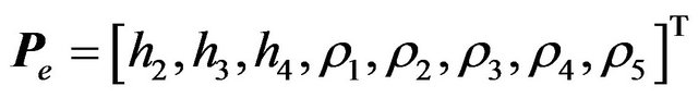
The scheme overview of joint inversion by [2] demonstrates the joint inversion of diverse subsurface electrical soundings and VSP (Vertical Seismic Profiling) measurements. The seismic model parameter vector is (the first and the fifth layers are considered to be half-spaces)
 , (1)
, (1)
where hi denotes the layer-thicknesses and vi denotes the seismic propagation velocities. The geoelectric model parameter vector is
 , (2)
, (2)
where ρi denotes the resistivities. The joint parameter vector 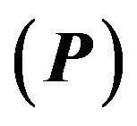 is the combination of vectors
  and
and 
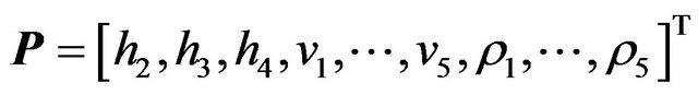 . (3)
. (3)
The common elements in the joint parameter vector in this example are the layer thicknesses as Equation (3) shows. The direct problem is
 , (4)
, (4)
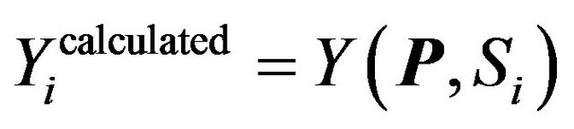
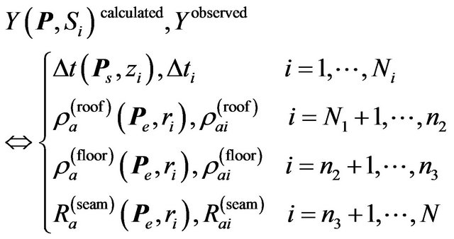
where S is a geometrical parameter S = z (depth) in seismic case and S = r (electrode spacing applied in underground electric measurement) in electric case. Joint inversion arises from the joint solution of non-linear functions
 (5)
(5)
where

and 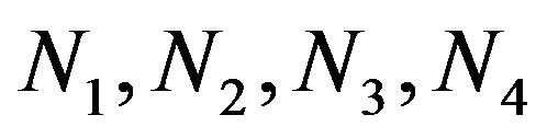 are the total numbers of seismic, roof, floor and seam sounding data, respectively, Δt is the travel-time difference between the travel-times measured by the seismic receivers (geophones),
 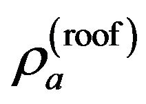 ,
, 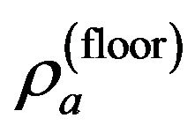 denotes the apparent resistivities in roof and floor sounding measurements, and
 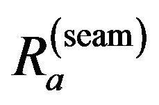 is the apparent resistance in the case of seam sounding measurement. The joint inversion involves the calculation of an appropriate parameter vector
  where quantities Ycalculated and Yobserved fit the best. Roof and floor sounding means soundings measured on different formation boundaries with identical arrays of the surface measurements. Seam sounding means a sounding measured with vertical dipole array in mine tunnels. The basic equation for the solution of the linearized inverse problem is
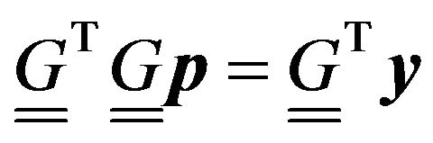 , (6)
, (6)
where  denotes the normalized model parameter vector dP/P,
  is the normalized data vector
(Yobserved‒Ycalculated)/Ycalculated and  is the Jacobi’s (sensitivity) matrix. Equation (5) presents that joint inversion makes use of one seismic and three types of geoelectric data sets. Roof and floor soundings provide different measured data sets because of the diversity of parameter sensitivities. Further geoelectric data measured in different arrays are involved in the joint inversion. One more seismic data set is attached to the previous data sets in the entire joint inversion. The data sets is different in three ways, i.e. in measurement array, in measurement (reference) level and physically different data sets are processed simultaneously in the inversion procedure, hence multiple joint inversion is realized.
2.1. The Role of Parameter Sensitivity in Joint Inversion
The definition of parameter sensitivity in geoelectric practice was given by Gyulai [3,4].
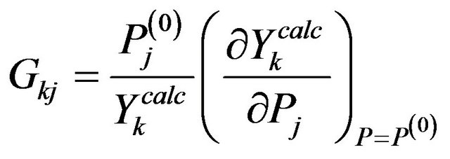 , (7)
, (7)
where  denotes the sensitivity of the k-th data with respect to the j-th parameter. The form of the Fischer Information Matrix [5] with the nominations of Equations (6) and (7) is
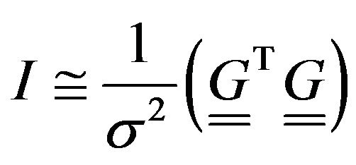 , (8)
, (8)
where 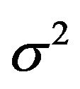 is the uncertainty (standard deviation of geophysical data) and
 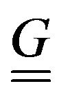 is the Jacobi’s matrix [6,7]. The Fischer Information matrix gives the possibility to quantify the information content of geophysical data related to the geological structure, which is used to decide whether the data sets are different. The diversity of data sets are joined to physical content that substantially affects the result of the inversion and explains the meaning of joint inversion.
It is questionable whether the joint inversion of similar measurements data results in any improvement in the parameter estimation or in the covariance matrix. The improvement is affected strongly by the data noise and the parameter sensitivities including the correlation between the parameter sensitivities as the biggest problem of the inversion. Generally we can state that if more complex the model then the application of the joint inversion is more required. The researches of our Department prove that the adequate joint inversion causes significant improvement of accuracy and reliability in case of 1D (1 Dimensional) model approximations. The selection of the measurement methods is based on the parameter sensitivities and noise tests. The next chapter presents a short overview about some typical case of joint inversion without striving for completeness.
2.2. Typical Cases of Joint Inversion
A common fact in geophysical exploration is that several measured data are connected to one station, e.g. VES (Vertical Electric Sounding) and magnetotelluric data. The simultaneous inversion of two different types of sounding data sets measured in the same station is joint inversion because of the diversity of their parameter sensitivities. If the data is duplicated according to the regular sampling then it does not signify joint inversion. The inversion of the average of VES data measured in dip and strike direction is a single inversion. In case of complex geological structures the symmetrization of the measurement array causes information loss depending on the approximation applied in the model dimension during the inversion.
The VES measurements are made with close spacing in both cases (29 VES stations in each section, 25 m away from each other). The difference between the two figures is due to measurements made by electrode spacings of various directions in the same station. One of the electrode spacing is made in “dip direction” (in direction of the shorter structural element in cross direction), the other is in “strike direction” (in direction of the longer structural element in straight direction). The joint inversion of dip and strike direction measurements has an advantage only in case of 2D (2 Dimensional) or 3D (3 Dimensional) structures. The information content of measurements in dip or strike direction significantly differs in this case as Figures 1 and 2 show. The complex model was built up of 2D and 3D elements and the distribution of resistivity sensitivities was calculated from VES data measured in Schlumberger array. Synthetic data were calculated with Spitzer’s algorithm [8]. The difference between the spatial and “along the profile” parameter sensitivities refers to the advantage that is provided by the simultaneous (joint) inversion. It is worth to look forward to the joint inversion of regional and “along the profile” measurements that are proposed to realize with series expansion based inversion.
The different orientations of the measurements eventuates differing data in case of anisotropic structures. Data derived from measurements with different directions open the door to simultaneous inversion. The previously mentioned simultaneous inversion can also be named as joint inversion.
In the recent the simultaneous inversion of data measured in different orientation (potential, gradient, dipoledipole array) is also joint inversion and it is especially referenced in cases of 2D and 3D structures.
Other various types of data sets can be derived from subsurface measurements where it is possible to measure the vertical derivates either in different depths besides the horizontal derivates or potentials (based on mine surveys measured in different levels and arrays by the Department of Geophysics). The simultaneous analysis of these data is also joint inversion.
Few decades ago it was a frequently used technique in
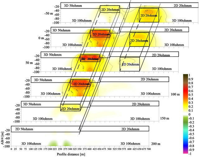
Figure 1. 3D parameter sensitivities of VES data measured in Schlumberger array in dip direction.
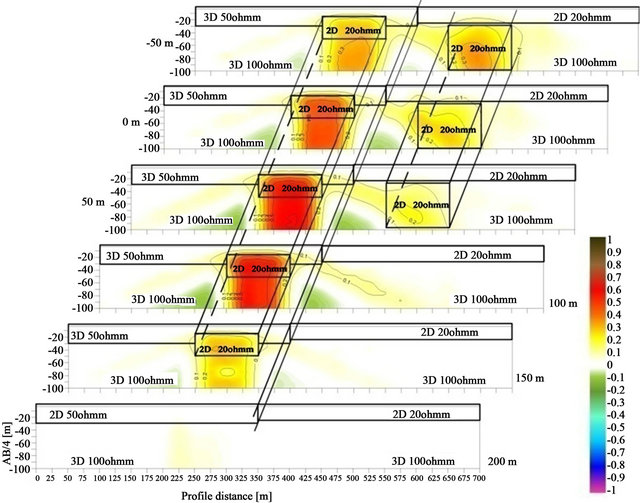
Figure 2. 3D parameter sensitivities of VES data measured in Schlumberger array in strike direction.
geoelectric exploration that the data sets of some measuring array, was transformed into another array [9,10]. The inversion results of the transformed data set show no difference from the inversion results of the original data sets. The reason is that the transformation does not increase the information content of the data because it also affects the noise rate and it possibly increases the parameter sensitivities together with the noises. According to this the simultaneous inversion of the original and transformed data sets is not a joint inversion.
Joint inversion can also be the inversion of only gravitational or only magnetic data measured in different reference levels [11]. In this case the simultaneous inversion of the original data and the one transformed into other levels cannot be accepted as joint inversion.
It is worthwhile to mention the time-lapse measurements used for the monitoring investigations in environmental geophysics where time dependence of physical properties of the structure is observed. The parameter sensitivity of time dependence means diverse information matrix which provides various type of data sets for the basis of a new type of joint inversion.
3. Special Case: Series Expansion Based Joint Inversion
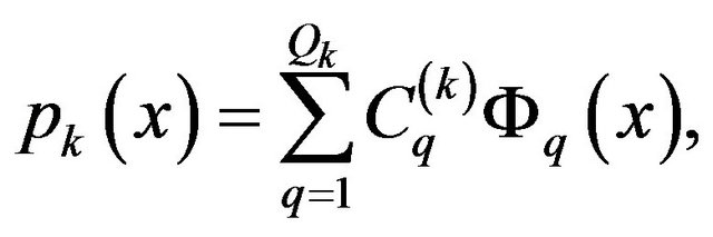
The series expansion based inversion method can be considered as a simultaneous inversion technique, where each data measured along a profile (or over an area) assists in the determination of the series expansion coefficients describing the geological structure [12-14]. The inversion technique allows to couple further data measured by different physical principles in one inversion procedure, which can improve the reliability of the interpretation results [15,16].
The principle of the series expansion based inversion method is that variations of layer boundaries and physical parameters along the profile are described by continuous functions. The discretization of model parameters is based on series expansion [17]
 (9)
(9)
where pk denotes the k-th physical or structural parameter , Cq is the q-th expansion coefficient and Φq is the q-th basis function (up to Q number of additive terms), which is the function of the independent variable x. Basis functions are known quantities, which may be chosen arbitrarily for the environmental geological setting. In earlier studies, it was demonstrated that geoelectric structures can be described properly by periodic basis functions [4,13].
In a simpler way a set of power basis functions can be used in Equation (9)
 . (10)
By this formulation all data measured along the profile are inverted simultaneously to determine the series expansion coefficients. The advantage of this technique is that the variation of structural and physical parameters can be described with significantly less unknowns (i.e. series expansion coefficients) than data, thus a highly overdetermined inverse problem is formulated, which is more favourable to solve than a marginally overdetermined or an underdetermined inverse problem. The strategy of choosing the number of expansion coefficients is detailed in Gyulai et al. [13].
In the inversion method the data of each VES station participate simultaneously in the determination of each coefficient hereby in the approximation of the parameters because the parameters of the structure are calculated from the coefficients. The determination of the structure with inversion method using series expansion means the simultaneous inversion of spatial data where the parameter sensitivities are different in each station. By our interpretation we consider this methodology a joint inversion approach. The simultaneous inversion of different data sets measured with different physical methods along the profile means further joint inversion based on the different measurements of orientation, lay-out of the array and reference levels and the different geophysical parameters. The further advantage of series expansion based inversion methods is the possibility of using joint inversion in case of not relevant boundaries. The unknowns of the inversion are the coefficients of the series expansion in Equation (9). In case of multi-layered models the condition of joint inversion is realized even if not all the layer-thicknesses fit to each other vice versa in every method. This term could also be fulfilled even if only a few coefficients are the same. For instance, the displacement of parallel boundaries can be described with the deviation of the constant coefficient while all the other coefficients fit to each other vice versa, thus still possible to perform “strong joint inversion”. Some common coefficients could be given often to different physical parameters that improves the result of the inversion. This possibility of inversion using series expansion was presented earlier [18] and the results were published [19].
4. Discussion and Conclusion
Consider the problem again what we could call various types of data sets that are inverted simultaneously. The general answer to this question could be given by referring to the information matrix. Those measurements could be called diverse where the Fischer Information Matrix is different to the data.
Wide range of the researches shows that there is intention for the application of joint inversion in the fields of geophysics [20-33].
We do not consider it a matter of principle in joint inversion that the various types of data sets are inverted simultaneously, receive nominations separately. Our opinion is that the best is to leave it to the practice. The posterior shows that standardized system evolves hardly and there are huge variances between the uses of the nominations. The definition of joint inversion often is limited to simultaneous inversion based on different physical principles. We prefer more the comprehensive application of joint inversion as far as possible numerical qualification based on physical principles and regarding to the accuracy of the approximation. We consider it especially relevant in environmental geophysics.
5. Acknowledgements
This described work was carried out as part of the TÁMOP-4.2.1.B-10/2/KONV-2010-0001 project in the framework of the New Hungarian Development Plan. The realization of this project is supplied by the European Union, co-financed by the European Social Fund. The authors are also grateful for the support of the research team of the Department of Geophysics, University of Miskolc.
REFERENCES
- K. Vozoff and D. L. B. Jupp, “Joint Inversion of Geophysical Data,” Geophysical Journal of the Royal Astronomical Society, Vol. 42, No. 3, 1975, pp. 977-991. doi:10.1111/j.1365-246X.1975.tb06462.x
- M. Dobróka, Á. Gyulai, T. Ormos, J. Csókás and L. Dresen, “Joint Inversion of Seismic and Geoelectric Data Recorded in an Underground Coal Mine,” Geophysical Prospecting, Vol. 39, No. 5, 1991, pp. 643-665. doi:10.1111/j.1365-2478.1991.tb00334.x
- Á. Gyulai, “Parameter Sensitivity of Underground DC Measurements,” Geophysical Transactions, Vol. 35, No. 3, 1989, pp. 209-225.
- Á. Gyulai and T. Ormos, “A New Procedure for the Interpretation of VES Data: 1.5-D Simultaneous Inversion Method,” Journal of Applied Geophysics, Vol. 41, No. 1, 1999, pp. 1-17. doi:10.1016/S0926-9851(98)00034-2
- P. Salát, Gy. Tarcsai, L. Cserepes, M. Vermes and D. Drahos, “Information-Statistical Methods of Geophysical Interpretation (in Hungarian),” Tankönyvkiadó, 1982.
- W. Menke, “Geophysical Data Analysis-Discrete Inverse Theory,” Academic Press, Inc., London, 1984.
- M. Dobróka, “Introduction to Geophysical Inversion (in Hungarian),” Miskolci Egyetemi Kiadó, Miskolc, 2001, 209 p.
- K. Spitzer, “A 3-D Finite Difference Algorithm for DC Resistivity Modelling Using Conjugate Gradient Methods,” Geophysical Journal International, Vol. 123, No. 3, 1995, pp. 902-914. doi:10.1111/j.1365-246X.1995.tb06897.x
- S. P. Dasgupta, “A Note on the Conversion of DC-Dipole Sounding Curves to Schlumberger Curves,” Geoexploration, Vol. 22, No. 1, 1984, pp. 43-45. doi:10.1016/0016-7142(84)90004-8
- R. Kumar and U. C. Das, “Transformation of Schlumberger Apparent Resistivity to Dipole Apparent Resistivity over Layered Earth by the Application of Digital Linear Filters,” Geophysical Prospecting, Vol. 26, No. 2, 1978, pp. 352-358. doi:10.1111/j.1365-2478.1978.tb01598.x
- Y. Li and D. W. Oldenburg, “Joint Inversion of Surface and Three Component Borehole Magnetic Data,” Geophysics, Vol. 65, No. 2, 2000, pp. 540-552. doi:10.1190/1.1444749
- M. Dobróka and L. Völgyesi, “Inversion Reconstruction of Gravity Potential Based on Gravity Gradients,” Mathematical Geosciences, Vol. 40, No. 3, 2008, pp. 299-311. doi:10.1007/s11004-007-9139-z
- Á. Gyulai, T. Ormos and M. Dobróka, “A Quick 2-D Geoelectric Inversion Method Using Series Expansion,” Journal of Applied Geophysics, Vol. 72, No. 4, 2010, pp. 232- 241. doi:10.1016/j.jappgeo.2010.09.006
- M. Kis, “Investigation of near Surface Structures with Joint Inversion of Seismic and Direct Current Geoelectric Data (in Hungarian),” Ph.D. Thesis, University of Miskolc, Miskolc, 1998.
- M. Dobróka and N. P. Szabó, “Combined Global/Linear Inversion of Well-Logging Data in Layer Wise Homogeneous and Inhomogeneous Media,” Acta Geodaetica et Geophysica Hungarica, Vol. 40, No. 2, 2005, pp. 203-214. doi:10.1556/AGeod.40.2005.2.7
- D. Drahos, “Inversion of Engineering Geophysical Penetration Sounding Logs Measured along a Profile,” Acta Geodaetica et Geophysica Hungarica, Vol. 40, No. 2, 2005, pp. 193-202. doi:10.1556/AGeod.40.2005.2.6
- M. Dobróka, “The Establishment of Joint Inversion Algorithms in the Well-Logging Interpretation (in Hungarian),” Scientific Report for the Hungarian Oil and Gas Company, University of Miskolc, Miskolc, 1993.
- Á. Gyulai, T. Ormos and L. Dresen, “A Joint Inversion Method to Solve Problems of Layer Boundaries, Differently Defined by Seismics and Geoelectric,” 6th Meeting of Environmental and Engineering Geophysical Society— European Section, 3-7 September 2000, Bochum.
- Á. Gyulai and T. Ormos, “New Geoelectric-Seismic Joint Inversion Method to Determine 2-D Structures for Different Layer Thickness and Boundaries,” Geophysical Transactions, Vol. 44, No. 3-4, 2004, pp. 273-300.
- M. Breitzke, L. Dresen, J. Csókás, Á. Gyulai and T. Ormos, “Paratmeter Estimation and Fault Detection by ThreeComponent Seismic and Geoelectrical Surveys in a Coal Mine,” Geophysical Prospecting, Vol. 35, No. 3, 1987, pp. 832-863.
- P. Dell’Aversana, “Joint Inversion of Seismic, Gravity and Magnetotelluric Data Combined with Depth Seismic Imaging,” EMG International Workshop, Capri, 2007.
- J. Doetsch, N. Linde, I. Coscia, S. A. Greenhalgh and A. G. Green, “Zonation for 3D Aquifer Characterization Based on Joint Inversions of Multimethod Crosshole Geophysical Data,” Geophysics, Vol. 75, No. 6, 2010, pp. G53-G64. doi:10.1190/1.3496476
- M. Dobróka, N. P. Szabó, E. Cardelli and P. Vass, “2D Inversion Borehole Logging Data for Simultaneos Fetermination of Rock Interfaces and Petrophysical Parameters,” Acta Geodaetica and Geophysica Hungarica, Vol. 44, No. 4, 2009, pp. 459-482. doi:10.1556/AGeod.44.2009.4.7
- L. A. Gallardo and M. A. Meju, “Joint Two Dimensional DC Resistivity and Seismic Traveltime Inversion with Cross-Gradients Contrains,” Journal of Geophysical Research, Vol. 109, No. B3, 2004, pp. B03311-B03321.
- L. A. Gallardo-Delagdo, M. A. Perez-Flores and E. Gomez-Trevino, “A Versatile Algorithm for Joint 3D Inversion of Gravity and Magnetic Data,” Geophysics, Vol. 68, No. 3, 2003, pp. 949-959. doi:10.1190/1.1581067
- E. Haber and D. Oldenburg, “Joint Inversion: A Structural Approach,” Inverse Problems, Vol. 13, No. 1, 1997, pp. 63-77. doi:10.1088/0266-5611/13/1/006
- A. Hering, R. Misiek, Á. Gyulai, T. Ormos, M. Dobróka and L. Dresen, “A Joint Inversion Algorithm to Process Geoelectric and Surface Wave Data, Part. I.,” Geophysical Prospecting, Vol. 43, No. 2, 1995, pp. 153-156. doi:10.1111/j.1365-2478.1995.tb00128.x
- M. Jegen, R. W. Hobbs, P. Tartis and A. Chave, “Joint Inversion of Marine Magnetotelluric and Gravity Data Incorporating Seismic Constrains. Preliminary Results of Sub-Basalt Imaging off the Farve Shelf,” Earth and Planetary Science Letters, Vol. 282, No. 1-4, 2009, pp. 47-95. doi:10.1016/j.epsl.2009.02.018
- N. Linde, A. Tryggvason, J. E. Peterson and S. S. Hubbard, “Joint Inversion of Crosshole Radar and Seismic Travel Times Acquired at the South Oyster Bacterial Transport Site,” Geophysics, Vol. 73, No. 4, 2008, pp. G29- G37. doi:10.1190/1.2937467
- G. F. Margrave, R. R. Steward and J. A. Larsen, “Joint PP and PS Seismic Inversion,” The Leading Edge, Vol. 20, No. 9, 2001, pp. 1048-1052. doi:10.1190/1.1487311
- R. Misiek, A. Liebig, Á. Gyulai, T. Ormos, M. Dobróka and L. Dresen, “A Joint Inversion Algorithm to Process Geoelectric and Surface Wave Seismic Data Part II,” Geophysical Prospecting, Vol. 45, No. 1, 1997, pp. 65-85. doi:10.1046/j.1365-2478.1997.3190241.x
- S. P. Sharma and S. K. Verma, “Solutions of the Inherent Problem of the Equivalence in Direct Current Resistivity and Electromagnetic Methods through Global Optimalisation and Joint Inversion by Successive Refinement of Model Space,” Geophysical Prospecting, Vol. 59, No. 4, 2011, pp. 760-776. doi:10.1111/j.1365-2478.2011.00952.x
- N. P. Szabó, “Global Inversion of Well-Logging Data,” Geophysical Transactions, Vol. 44, No. 3-4, 2004, pp. 313- 329.