Open Journal of Optimization
Vol.2 No.3(2013), Article ID:35957,8 pages DOI:10.4236/ojop.2013.23008
Multicriteria Optimization of Cellular Networks
1Institute of Machines Science Named after A. A. Blagonravov of the Russian Academy of Sciences, Moscow, Russia
2Department of Information Sciences, Naval Postgraduate School, Monterey, USA
3Central Institute of Aviation Motors Named after P. I. Baranov, Moscow, Russia
4Center for Health Informatics and Bioinformatics, New York University Medical Center, New York, USA
Email: Alexander.Statnikov@med.nyu.edu
Copyright © 2013 Roman Statnikov et al. This is an open access article distributed under the Creative Commons Attribution License, which permits unrestricted use, distribution, and reproduction in any medium, provided the original work is properly cited.
Received May 28, 2013; revised June 25, 2013; accepted July 9, 2013
Keywords: Feasible Solution Set; Pareto Optimal Solutions; Parameter Space Investigation (PSI) Method; Cellular Networks; Multicriteria Problems
ABSTRACT
When designing modern cellular networks, it is challenging to account for many contradictory criteria and constantly changing external conditions of the networks (e.g., traffic). We need to solve multicriteria problems with high-dimensional vectors of parameters. A prerequisite to solution of these problems is correct determination of the feasible solution set, which is directly related to the statement of optimization problem. This is a major challenge in all multicriteria engineering optimization problems and represents significant difficulties for the expert. In this paper, we show how to define the feasible solution set for cellular network optimal design problems and thus answer the fundamental question of where to search for optimal solutions in such problems. We use the Parameter Space Investigation (PSI) method implemented in the Multicriteria Optimization and Vector Identification (MOVI) software system and apply it to a mathematical model of cellular network. In addition to developing methodology for stating and solving the problem of multicriteria optimization of cellular network, we have found that 1) defining the feasible solution set is directly related to the correct statement of the optimization problem, 2) once the feasible solution set has been determined, the criteria convolution can be applied to find the optimal solution in the feasible solution set, 3) it is possible to perform online tuning of the cellular network parameters.
1. Introduction
One of the distinguishing characteristics of cellular networks is difficulty of their design given a large number of contradictory criteria and constantly changing external conditions of the networks (e.g., traffic). In addition to multiple criteria, we deal with vectors of parameters of high dimensionality (hundreds to thousands). Optimal design of cellular networks is at the interface of design and management problems, and there have hardly been any attempts to construct a feasible solution set for problems of such type. The feasible solution set is essential because it contains a Pareto set of optimal solutions, none of which can be improved along all quality criteria simultaneously. In addition to the difficulties in determining the feasible solution set, choice of the best solution from a Pareto set is also non-trivial when this set contains a large number of solutions. In some cases, these difficulties can be mitigated by applying criteria convolution as described below. However, in order to apply convolutions correctly, one has to define feasibility of obtained solution first, which makes a proper construction of the feasible solution set the key factor. In this work, we consider applying the Pareto Space Investigation (PSI) method as an attempt to improve existing techniques of network design and management by constructing and analyzing the feasible solution set. The goal of this paper is to show feasibility and capabilities of the PSI method for solving problems of optimal design of cellular networks.
Most existing works on cellular network optimization that deal with multi-criteria problems transform them into single-objective variant using some scalarization techniques [1,2], weighted sum being the most popular approach. Melachrinoudis and Rosyidi [3] use simulated annealing algorithm to optimize weighted sum of three criteria (call quality, demand coverage and total cost) by varying location, power and antenna height of base stations. Galota et al. [4] choose positions of base stations to optimize weighted sum of three criteria (number of supplied demand nodes, ongoing costs, and cost of intra-cell interference) subject to constraint on construction costs. Amaldi et al. [5] aim at maximizing total covered traffic and minimizing total installation costs by forming weighted sum of these criteria; two-stage Tabu Search algorithm is used starting from solution provided by randomized greedy procedure. Hurley [6] proposes framework based on Simulated Annealing for optimization of objective function that is sum of five criteria (coverage, site cost, traffic, interference, and handover). Gerdenitsch [7] uses sum of number of served users, coverage, and soft handover as objective function for the problem of tuning transmit power and antenna downtilt using Genetic Algorithm. Zhu and Buot [8] propose heuristic algorithm for online network optimization based on estimating linear model between KPIs (key performance indicators) and parameters (expressed in form on sensitivity matrix) from a-priori simulation results and KPI measurements. Weighted sum of five KPIs is used as optimization process performance index. The approach allows specifying KPI targets.
In few works ε-constraint technique is utilized: one of criteria is selected to be optimized, and others are converted into constraints [1,2]. One of network optimization problems studied by Siomina [9] is example of such approach: total network load (total pilot power) is minimized subject to coverage constraint. Other approaches not based on some form of scalarization (weighted sum or ε-constraint) are much less common. Jedidi et al. [10] argue that it makes sense to consider cells overlap and cells geometry as criteria for real-life network optimization. They aim at finding the whole Pareto front of this bi-criteria problem using a version of Multiobjective Evolutionary Algorithm. It is well known that such algorithms are quite effective for two or three criteria problems, as higher number of criteria their applicability is an open question [11]. To the best of our knowledge, most commercial cellular network planning and optimization tools are also based on some form of scalarization such as weighted sum [12,13].
2. Problem Formulation
In this paper, we are concerned with multicriteria optimization problems arising during planning and operation of cellular mobile network. Mobile network provides service in area divided into cells, each served by transceiver of base station that has several tunable parameters affecting network performance like transmit power, antenna orientation, associated radio frequency, parameters of radio resource management algorithms, etc. Typically these parameters are configured by experts (possibly with the help of network planning and optimization tools) during network planning stage and kept fixed for a long period of time. Cellular network demand and environment are ever changing during day, and such fixed configuration (usually targeted at peak network load-busy hour) can become not well suited for current network conditions. It is also possible to change some of cellular network parameters online trying to adapt to changing conditions. Thus network optimization can be performed in offline (with full set of parameters available for configuration and lots of time for decision making) or online (with restricted set of parameters available and limited time for decision making) mode. We propose using of the Parameter Space Investigation method in both of the network optimization modes.
Reference signal transmit power and antenna electrical downtilt are one of the most important parameters that have great impact on different network KPIs such as capacity and coverage. Moreover, these two parameters can be changed remotely and automatically as opposed to manual and costly reconfiguration of some other important parameters (such as antenna azimuth or mechanical downtilt). This is the motivation for using the above two parameters for our study.
Whole network area is divided into pixels using some grid (typical size is 50 m ´ 50 m), each pixel is characterized by receive power level from each cell in network and mean number of users in it. The former aggregates into signal propagation maps (one for each cell), and the latter into traffic map (traffic maps can be differentiated by type of service). Reference signal received power is reference signal transmit power times channel gain between cell and pixel, influenced by antenna downtilt of this cell. Increasing transmit powers of all cells and pointing antennas up (corresponds to small downtilt values), we increase coverage in network (received power in each pixel becomes high enough to connect to the cell with strongest signal) but at the same time we increase interference between cells, which effectively leads to network capacity degradation. Trade-off between these objectives is not obvious, and needs to be carefully studied. It is hard to say beforehand what KPI values are achievable [12-15].
2.1. System Model
Let us denote by c = 1, …, С the set of cells serving planning area represented by a grid of pixels. Signal propagation (averaged in time and frequency) from each cell c to each pixel m is characterized by power gain gmcAmc, composed of isotropic gain gmc and antenna gain Amc. Antenna gain Amc depends on electrical downtilt tc of antenna associated with cell c and direction (given by azimuth fmc and elevation qmc angles) between this antenna and pixel m: , where Gc is cell’s c antenna maximum gain,
  and
and  are tabulated functions of horizontal and vertical cell c antenna patterns [14].
Reference Signal Received Power (RSRP) Rmc from cell c in pixel m is calculated as
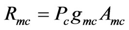 where Pc is reference signal transmit power of cell c.
Each pixel m is associated with cell c with largest received power Rmc among all other cells, for such pixel– cell pair m, c we set association indicator amc equal to 1. Signals from all other cells interfere with useful signal from serving cell. One of the most important link quality indicators is Reference Signal Signal-toInterference and Noise Ratio (RSSINR) given by
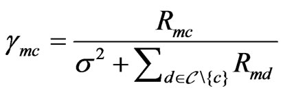 where
where  is noise power.
Each cell has frequency resources (resource blocks in LTE) that it allocates between served users. We use definition of cell load as long-term average percentage of utilized frequency resources [16]. Cell load depends on amount of traffic requested by served users and their link capacities. We characterize long-term average requested traffic in pixel m using Tm—average number of users in this pixel requesting some service, and D—bitrate demand of this service. Load of cell c required to serve its users is estimated as
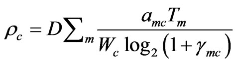 where Wc is bandwidth of frequency resources available in cell c. Here we used Shannon formula for link capacities.
2.2. Performance Criteria
Call Drop and/or Block Rate (CDBR) performance criterion FCDBR is determined by cell loads and number of served users as
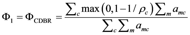 .
.
Percentage of RSRP and RSSINR covered area criteria FRSRP-covA and FRSSINR-covA are defined as

and
 where
where  and
and  are RSRP and RSSINR thresholds and
 . In a similar way percentage of RSRP and RSSINR covered traffic criteria criteria FRSRP-covT and FRSSINR-covT are defined as
 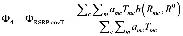 and
and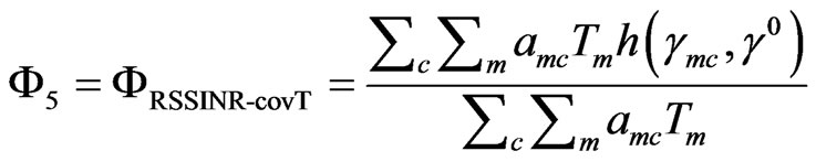 . Mean SINR
(Signal to Interference and Noise Ratio) [dB] KPI is defined as 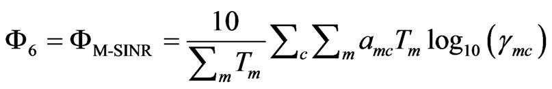 .
.
Mean required cell load criterion is 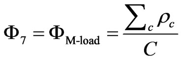 . Aggregated criterion is weighted sum of the above seven criteria
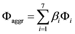 . Usually cellular network operator has well-defined targets that should be achieved for RSRP-covA, RSRP-covT, and CDBR criteria, and additionally we would like to maximize/minimize the following criteria shown in Table 1.
In our examples, we consider network consisting of 50 cells with 100 variables. Variables are transmit power pc and electrical downtilt tc, c = 1, ..., 50. The considered network with traffic map is shown in Figure 1. In the
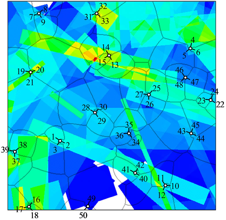
Figure 1. Map of cellular network used in examples. Color intensity corresponds to traffic map (ranging from blue– small number of users, to red–large). Base stations are located at white dots, each having three antennas (one antenna serves one cell). Short black line segments represent horizontal direction of corresponding antennas. Numbers are cell indices. Grey lines are cell borders. For example cells with indices 10, 11, and 12 are served by transceivers of one base station, antenna of cell 10 is directed towards East, 11—Northwest, and 12—Southwest.

Table 1. Criteria names, meaning and objective.
first problem (Task 1), 0 £ pc £ 40 W, 0˚ £ tc £ 10˚ of each cell, c = 1, ..., 50. In the second problem (Task 2), 0 £ pc £ 50 W. The ranges of change for the electrical downtilt are kept unchanged by 0˚ £ tc £ 10˚ of each cell, c = 1, ..., 50. Electrical downtilt constraints are determined by capabilities of antennas serving each cell. Transmit power constraints are also due to hardware limitations (power amplifier) and electromagnetic radiation regulations.
In what follows we will show how to construct the feasible solution set for the above set of performance criteria.
3. Construction of the Feasible and Pareto Optimal Solution Sets
3.1. Generalized Formulation of Multicriteria Optimization Problems
We discuss here a mathematical formulation that can be applied to the majority of engineering optimization problems [17-23]. In the general case, when designing a system, one has to take into account the design variable constraints, the functional constraints, and the criteria constraints.
The design variable constraints (constraints on the design variables) have the form:
 (1)
(1)
The functional constraints on functional dependences fl(a) may be written as follows:
 (2)
(2)
where  and
and  are, respectively, the lower and the upper admissible values of the quantity fl(a). Conditions (2) often represent compliance with standard regulatory requirements to the system. As a rule, vectors of design variables
  are calculated using uniformly distributed sequences. In the present case, a random number generator was applied because of high dimensionality of the design variable space.
There also exist particular performance criteria. It is desired, all other things being equal, these criteria, denoted by  take the extreme values. For simplicity, we assume that
  are to be minimized.
The constraints (1) single out a parallelepiped P in the r-dimensional design variable space (space of design variables).
In order to avoid situations, in which the expert regards the values of some criteria as unacceptable, we introduce the criteria constraints
 (3)
(3)
where  is the worst value of the criterion
  to which the expert may agree. The choice of
  is discussed in what follows.
The criteria constraints differ from the functional constraints in that the former are determined when solving a problem and, as a rule, are repeatedly revised. Hence, unlike  and
and , reasonable values of
  cannot be chosen before solving the problem.
Constraints (1)-(3) define the feasible solution set D.
If the functions fl(a) and  are continuous in P, then the sets G and D are closed.
Now let us formulate one of the basic problems of multicriteria optimization. It is necessary to find such a set P Ì D for which
 (4)
(4)
where  is the criterion vector and P is the Pareto optimal set.
In other words, a point , is called a Pareto optimal point iff there exists no point
  such that
  for all n = 1, …, k and
  for at least one n Î {1, …, k}. A set P Ì D is called the Pareto optimal set iff it consists of Pareto optimal points.
The Pareto optimal set plays an important role in vector optimization problems, because it can be analyzed relatively easier than the feasible solution set and because, by definition, the optimal vector always belongs to the Pareto optimal set, irrespective of the system of preferences used by the expert for comparing vectors belonging to the feasible solution set.
Very often, the experts do not encounter serious difficulties in analyzing the feasible solution set and the optimal set and in choosing the most preferred solution. They have a sufficiently well-defined system of preferences. Moreover, the aforementioned sets usually contain a small number of elements [17,23].
3.2. The PSI Method
To formulate and solve engineering optimization problems, the Parameter Space Investigation (PSI) method has been developed. According to this method, in the process of dialogues with a computer, the expert determines the criteria constraints and performs multicriteria analysis. The PSI method gives the expert valuable information on the advisability of revising various criteria, functional, and design variable constraints with the aim of improving the basic criteria. The expert sees what price one pays for making concessions in various criteria, i.e., what one loses and what one gains. In other words, the expert corrects initial problem statement while solving it, analyses the feasible solution set, and then makes a decision. A systematic and comprehensive description of the method can be found in [17,21,23].
After analyzing P (Pareto optimal set), the expert finds the most preferred solution . Typically, for the problems under consideration, experts do not have serious difficulties in analyzing the Pareto optimal set and in choosing the most preferred solution. Thus, the PSI method has proved to be a very convenient and effective tool for the expert, primarily because this method can be directly used for the statement and solution of the problem in an interactive mode. The PSI method is implemented in the Multicriteria Optimization and Vector Identification (MOVI) software system [17].
It is also worth mentioning that while there are many optimization methods, the PSI method more fully addresses characteristics of real-world engineering optimization problems (e.g., multiple criteria, difficulties in determining constraints on design variables, functional dependences and criteria) and allows the expert to simultaneously formulate and solve them in an interactive mode.
4. Application of the PSI Method to Improving the Network
The PSI method has been applied to the mathematical model of the network described above. Recall that in the above two examples, we have 50 cells with 100 variables and the number of criteria is seven. As test examples, we solve Task 1 and Task 2, that differ in maximum allowed transmit power—40 W and 50 W, respectively.
4.1. Test Tables for Task 1 (40 W)
As follows from the PSI method, the criteria constraints should be determined first. We have constructed the test table after 10,000 tests, see Table 2. The list of criteria, the best and worst values of criteria are shown in the
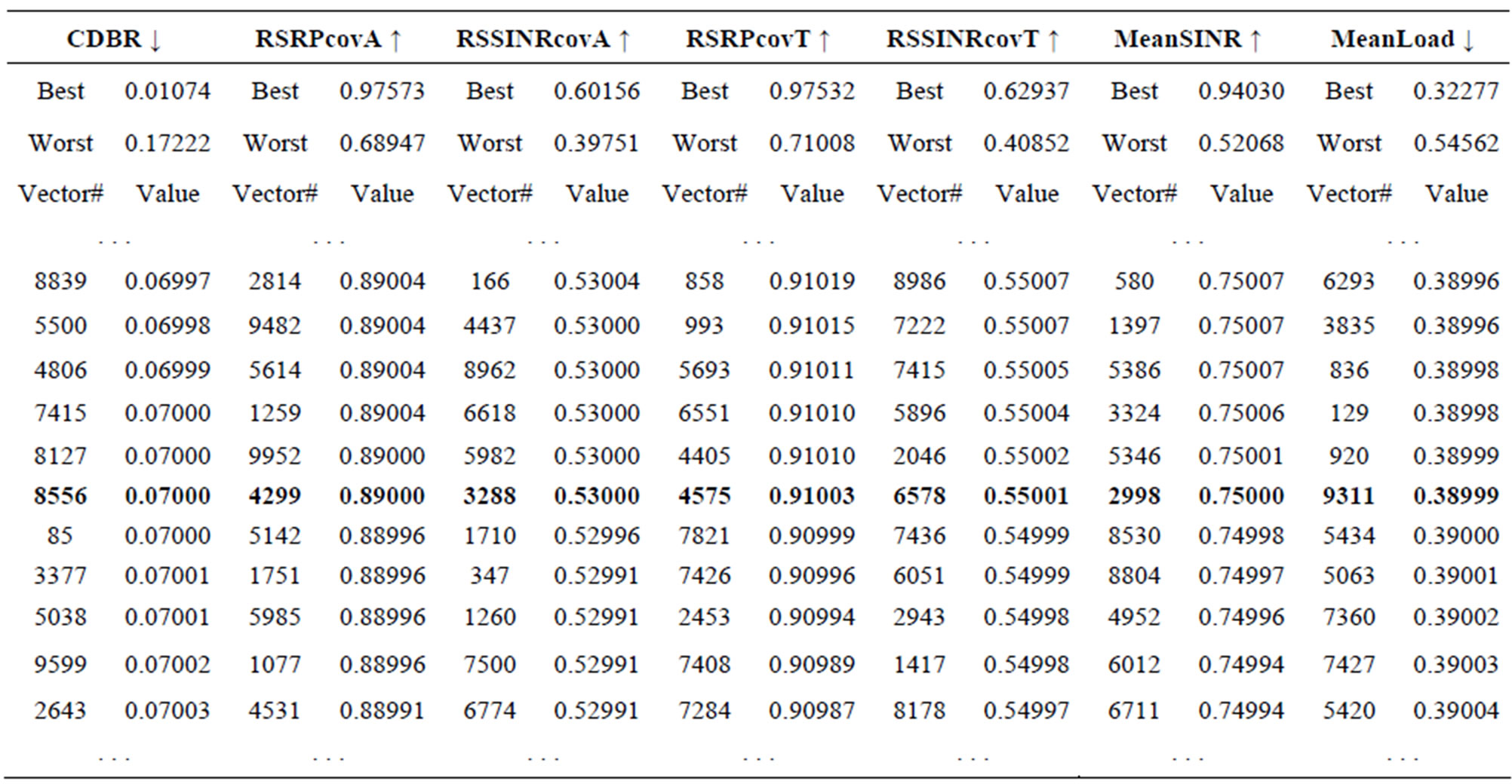
Table 2. Fragment of the tеst tables (Criteria that maximized and minimized are denoted with and ¯, respectively).
first, second and third rows, respectively. As a result of the dialogues of computer with the expert, the criteria constraints (0.07000; 0.89000; 0.53000; 0.91003; 0.55001; 0.75000; 0.38999) have been determined, see Table 2. We have obtained 256 feasible solutions, including 50 Pareto optimal solutions. Since these constraints met the expert’s requirements, they have been accounted for in all further studies. These constraints were identical in Task 2 (50 W), where we have conducted 10,000 tests and obtained 2867 feasible solutions, including 95 Pareto optimal solutions.
4.2. Criteria Histograms for Task 1
Criteria histograms are constructed on the basis of test tables and allow us to make a decision based on the obtained values of the criteria vectors and their significance [17,23]. In particular, the histograms allow us to correct the initial problem statement and reveal criteria relations. Histograms show Pareto optimal vectors for all criteria (e.g., see Figure 2). For each criterion, a horizontal line is assigned, along which vertical bars are plotted. Each bar corresponds to a vector from the Pareto optimal set. The location of each bar is defined by a corresponding criterion value for this vector. Criterion name as well as the worst and best criterion values are displayed to the left and to the right of the corresponding horizontal band, respectively.
Figure 2 shows locations of all 50 Pareto optimal vectors within obtained constraints on their values. Each of 50 solutions is uniquely colored. As can be seen, improving some criteria leads to deterioration of the others. For example, Pareto optimal solution #2544 is the best according to the fourth criterion (RSRP-covT,  = 0.9708) and one of the best according to the second criterion (RSRP-covA,
  = 0.9535) however it is the worst according to the seventh criterion (Mload,
  = 0.3868) and one of the worst according to the third (RSSINR-covA,
  = 0.5355), fifth (RSSINR-covT,
  = 0.5533), and sixth (MeanSINR,
  = 0.7692) criteria, (see Figure 2). These histograms demonstrate complex relationships that exist between the criteria.
4.3. Search for Optimal Solutions by Optimization of the Criteria Aggregate
In our case, the biggest challenges for an expert included the choice of a preferred solution from the Pareto optimal set: there were 50 and 95 Pareto optimal solutions in Task 1 and Task 2, respectively. As mentioned above, an expert defined an objective function as an aggregate of criteria

where b1 = 0.2, b2 = –0.2, b3 = –0.1, b4 = –0.2, b5 = –0.1, b6 = –0.1, and b7 = 0.1. The search for optimal solution was performed on the feasible set which is defined by constraints on parameters and criteria. For Task 1, the minimal value of the criteria aggregate (see [24]) was –0.6226, with the vector of criteria (0.0072; 0.9804; 0.6803; 0.9827; 0.7207; 1.1813; 0.2676). For Task 2, the minimal value of the criteria aggregate was –0.6262 with the vector of criteria (0.0108; 0.9748; 0.6825; 0.9819; 0.7275; 1.2209; 0.2612).
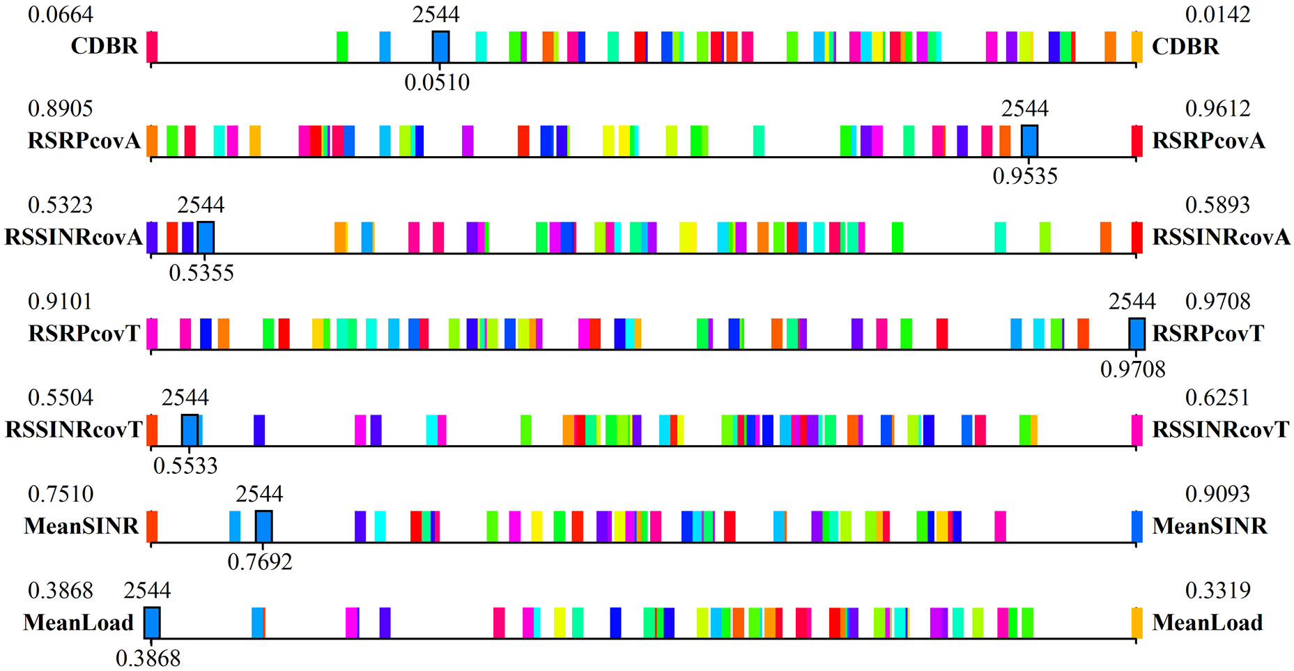
Figure 2. Criteria histograms. Location of the vector #2544. See text for details.
5. Conclusions
The conclusions of this work are three-fold. First, defining the feasible solution set is directly related to the correct statement of the optimization problem for the cellular network. We developed methodology for stating and solving the problems of multicriteria optimization for cellular network and showed how to state and solve the multicriteria problem of construction of the feasible and Pareto optimal solution sets.
Second, as it is known, the most preferable solution is determined on the Pareto set. In order to find it, one has to determine feasible solution set. Determination of the latter, correct definition of criteria constraints, turned out to be a difficult problem. These constraints were determined as a result of dialogues between an expert and compute while analyzing the test tables. Analysis of the Pareto optimal set is also challenging for the expert because of a large number of Pareto solutions. To overcome this, we have used a convolution of criteria. It is worthwhile to note that only after the feasible solution set has been determined, the criteria convolution can be successfully applied to find the optimal solution.
Third, to tune the network parameters online, i.e. to account for real distribution of the traffic, the operator may reduce the time required for the analysis. This process can be automated.
6. Acknowledgements
The authors are grateful to M. Pikhletsky (National Research University “Moscow Power Engineering Institute”) for participation in the problem formulation. The authors would like to thank A. Isyanov (Central Institute of Aviation Motors) for his contribution to computational experiments.
REFERENCES
- K. Miettinen, “Nonlinear Multiobjective Optimization,” Kluwer, Boston, 1999.
- J. Branke, K. Deb, K. Miettinen and R. Slowinski, “Multiobjective Optimization: Interactive and Evolutionary Approaches,” Springer-Verlag, Berlin, 2008. doi:10.1007/978-3-540-88908-3
- E. Melachrinoudis and B. Rosyidi, “Optimizing the Design of a CDMA Cellular System Configuration with Multiple Criteria,” Annals of Operations Research, Vol. 106, No. 1-4, 2001, pp. 307-329. doi:10.1023/A:1014574028174
- M. Galota, C. Glaßer, S. Reith and H. Vollmer, “A Polynomial-Time Approximation Scheme for Base Station Positioning in UMTS Networks,” Proceedings of the 5th International Workshop on Discrete Algorithms and Methods for Mobile Computing and Communications, Rome, 21 July 2001, pp. 52-59.
- E. Amaldi, P. Belotti, A. Capone and F. Malucelli, “Optimizing Base Station Location and Configuration in UMTS Networks,” Annals of Operations Research, Vol. 146, No. 1, 2006, pp. 135-151. doi:10.1007/s10479-006-0046-3
- S. Hurley, “Planning Effective Cellular Mobile Radio Networks,” IEEE Transactions on Vehicular Technology, Vol. 51, No. 2, 2002, pp. 243-253. doi:10.1109/25.994802
- A. Gerdenitsch, “System Capacity Optimization of UMTS FDD Networks,” PhD Thesis, Technische Universitat Wien, Wien, 2004.
- H. Zhu and T. Buot, “Multi-Parameter Optimization in WCDMA Radio Networks,” Vehicular Technology Conference, Milan, 17-19 May 2004, pp. 2370-2374.
- I. Siomina, “Radio Network Planning and Resource Optimization: Mathematical Models and Algorithms for UMTS, WLANs, and Ad Hoc Networks,” PhD Dissertation, Linkoping University, Linkoping, 2007.
- A. Jedidi, A. Caminada and G. Finke, “2-Objective Optimization of Cells Overlap and Geometry with Evolutionary Algorithms,” Applications of Evolutionary Computing, Lecture Notes in Computer Science, Vol. 3005, 2004, pp 130-139.
- V. Khare, X. Yao and K. Deb, “Performance Scaling of Multi-Objective Evolutionary Algorithms,” Proceedings of the Second Evolutionary Multi-Criterion Optimization (EMO-03) Conference (LNCS 2632), Faro, 8-11 April 2003, pp. 376- 390.
- Symena Software and Consulting GmbH. “CAPESSO 14.3 User Manual,” 2011.
- Forsk SA, “Atoll 2.8.3-User Manual,” 2010.
- U. Turke, “Efficient Methods for WCDMA Radio Network Planning and Optimization,” PhD Dissertation, TeubnerVerlag and DeutscherUniversitats-Verlag, Wiesbaden, 25 September 2007.
- H. F. Geerdes, “UMTS Radio Network Planning: Mastering Cell Coupling for Capacity Optimization,” PhD Dissertation, Technische Universitat Berlin, Berlin, 2008.
- K. Majewski and M. Koonert, “Conservative Cell Load Approximation for Radio Networks with Shannon Channels and Its Application to LTE Network Planning,” IEEE Sixth Advanced International Conference on Telecommunications, Barcelona, 9-15 May 2010.
- R. Statnikov and A. Statnikov, “The Parameter Space Investigation Method Toolkit,” Artech House, Boston/London, 2011.
- R. Statnikov and J. Matusov, “Multicriteria Analysis in Engineering,” Kluwer Academic Publishers, Dordrecht/ Boston/London, 2002. doi:10.1007/978-94-015-9968-9
- R. Statnikov and J. Matusov, “Multicriteria Optimization and Engineering,” Chapman & Hall, New York, 1995. doi:10.1007/978-1-4615-2089-4
- R. Statnikov, “Multicriteria Design. Optimization and Identification,” Kluwer Academic Publishers, Dordrecht/ Boston/London, 1999. doi:10.1007/978-94-017-2363-3
- I. M. Sobol’ and R. B. Statnikov, “Selecting Optimal Parameters in Multicriteria Problems,” 2nd Edition, Drofa, Moscow, 2006 (in Russian).
- R. B. Statnikov and J. B. Matusov, “Use of Nets for the Approximation of the Edgeworth-Pareto Set in Multicriteria Optimization,” Journal of Optimization Theory and Application, Vol. 91, No. 3, 1996, pp. 543-560. doi:10.1007/BF02190121
- R. Statnikov, J. Matusov and A. Statnikov, “Multicriteria Engineering Optimization Problems: Statement, Solution and Applications,” Journal of Optimization Theory and Applications, Vol. 155, No. 2, 2012, pp. 355-375. doi:10.1007/s10957-012-0083-9
- B. Suman and P. Kumar, “A Survey of Simulated Annealing as a Tool for Single and Multiobjective Optimization,” Journal of the Operational Research Society, Vol. 57, 2006, pp. 1143-1160. doi:10.1057/palgrave.jors.2602068