Open Journal of Optimization
Vol.2 No.4(2013), Article ID:40368,14 pages DOI:10.4236/ojop.2013.24013
Multi-Objective Optimization of Low Impact Development Designs in an Urbanizing Watershed
1Tetra Tech, Inc., Fairfax, USA
2Department of Agricultural and Biological Engineering, Pennsylvania State University, University Park, USA
3Department of Civil and Environmental Engineering, Pennsylvania State University, University Park, USA
4Bechtel Co., Houston, USA
Email: *guoshun.zhang@tetratech.com, hyc@psu.edu, preed@engr.psu.edu, yongnat@gmail.com
Copyright © 2013 Guoshun Zhang et al. This is an open access article distributed under the Creative Commons Attribution License, which permits unrestricted use, distribution, and reproduction in any medium, provided the original work is properly cited.
Received September 21, 2013; revised October 29, 2013; accepted November 15, 2013
Keywords: Multi-Objective Optimization; ε-NSGAII; Low Impact Development; SWMM; Stormwater
ABSTRACT
Multi-objective optimization linked with an urban stormwater model is used in this study to identify cost-effective low impact development (LID) implementation designs for small urbanizing watersheds. The epsilon-Non-Dominated Sorting Genetic Algorithm II (ε-NSGAII) has been coupled with the US Environmental Protection Agency’s Stormwater Management Model (SWMM) to balance the costs and the hydrologic benefits of candidate LID solutions. Our objective in this study is to identify the near-optimal tradeoff between the total LID costs and the total watershed runoff volume constrained by pre-development peak flow rates. This study contributes a detailed analysis of the costs and benefits associated with the use of green roofs, porous pavement, and bioretention basins within a small urbanizing watershed in State College, Pennsylvania. Beyond multi-objective analysis, this paper also contributes improved SWMM representations of LID alternatives and demonstrates their usefulness for screening alternative site layouts for LID technologies.
1. Introduction
Urban growth is often associated with increased runoff volume and peak flow rate, as well as reduced groundwater recharge and deteriorated downstream water quality [1]. Traditional engineering practices to manage the adverse hydrologic and water quality impacts of urbanization have relied on structural best management practices (BMPs) (e.g., detention and retention basins), which are often placed at a downstream location and provide centralized treatment [2]. Low impact development (LID) is a relatively new, and an increasingly popular, concept in stormwater management for controlling adverse storm flows and water quality impacts of urban sprawl [3,4]. The LID approach employs distributed small-scale, onsite, integrated management practices (IMPs; e.g. bioretention areas, green roofs, porous pavements, grass swales, etc.) to treat and infiltrate runoff at the source. The overall goal of LID practices is to create a hydrologically functional landscape that mimics the predevelopment watershed runoff conditions [5]. Over the last decade, LID practices have been utilized in urban stormwater management design in the United States by an increasing number of design engineers, municipalities, states, and federal agencies [3,6-9].
Despite the rapid growth of the LID approach, the quantification of storm flow reductions and water quality benefits from LIDs are still largely empirical. This is mainly due to the inherent uncertainty associated with the wide range of analysis techniques used to assess these small-scale management practices, especially when they are implemented collectively over a range of site conditions [10]. In order to assist engineers to appropriately design and evaluate LID implementation schemes, various BMP performance databases have been developed to serve as references [11,12]. Since the BMP databases are in their infancy with limited records and subsequently make the match between a site study and a database record difficult, most BMP modeling efforts have relied upon standard BMP performance values from the literature [13-15] to assess the aggregated hydrologic and/or water quality benefits. The LID designs based on these literature performance values, however, could be either over-sized or under-sized if specific conditions of the study site vary from the conditions where the literature performance values are obtained.
Cost-effective implementations of stormwater management strategy always require the identification of tradeoff between water quantity and quality benefits and the total IMP costs. For example, optimization of detention pond and land use planning was carried out by Harrell and Ranjithan [16], using a simple genetic algorithm (GA) to generate a cost effective detention pond configuration within subcatchments of a watershed to meet water quality control targets. Zhen et al. [17] investigated the optimization of location and sizing of stormwater detention basins at the watershed scale. They utilized the scatter search (SS) method to optimize detention basin designs for a series of pollutant reduction percentages, in order to obtain the tradeoff between the total costs and the potential reductions provided by the basins. In order to estimate the tradeoff between peak flow reduction and BMP cost for generic infiltration type BMPs, Perez-Pedini, et al. [1] linked a genetic algorithm to a simplified hydrologic model that is based on the NRCS curve number (CN) method. The tradeoff was generated by repeatedly solving the optimization problem over a range of project costs [1].
Optimization can be run using either design storm or the continuous simulation methods. For example, Harrell and Ranjithan [16] used the annual total rainfall excess during the optimization of wet detention ponds in City Lake watershed in High Point, North Carolina. PerezPedini, et al. [1] used a historical real event to optimize generic BMPs in the Aberjona River watershed near Boston, Massachusetts. While the design storm approach is mainly used for evaluations of hydrologic benefits, the continuous simulations are more frequently used for assessment of water quality related benefits [18]. Zhen, et al. [17] used a three-year simulation when optimizing detention BMPs for maximum sediment removal. Giatu, et al. [19] carried out ten-year simulations in Town Brook watershed, Delaware County, New York for the optimization of Phosphorous load reduction through BMPs. A fifteen-year continuous simulation was used when Maringanti, et al. [20] optimized the BMP implementations in L’Anguille River Watershed, Arkansas for phosphorrous load reduction.
The last several years have witnessed a rapid evolvement of optimization frameworks in watershed management. Two prominent examples are the BMP Decision Support System for the Prince George’s County, Maryland (PGBMPDSS) [21] and the US Environmental Protection Agency (USEPA)-approved System for Urban Stormwater Treatment and Analysis Integration (SUSTAIN) [22]. Both of the systems are capable of carrying out optimization analysis on a variety of BMPs to meet hydrologic and water quality management objectives. Hydrologic and water quality simulation algorithms in the two systems are similar to those in the USEPA Stormwater Management Model (SWMM), and the optimization techniques of GA and SS are available in the systems. The PGBMPDSS and SUSTAIN systems have been successfully implemented in numerous studies around the country in assisting informed stormwater management [23,24]. One potential limitation of the two systems is that both systems run on the ArcGIS platform, which requires frequent updates.
To date, no optimization framework has been developed to directly integrate the SWMM model with an optimization algorithm in carrying out cost-effective stormwater management analyses. One of the major hindrances to this is the representation of LID modules in SWMM [10], which has not been available until in recently updated version (Version 5.0.022) of the model. With the fact that the LID modules are relatively new and verification studies of the modules are still growing, our previously verified LID representation schemes in an earlier version of the SWMM model (Version 5.0.018) are coupled with an optimization algorithm in this study to form an optimization framework. The simulation-optimization framework is then demonstrated at the urbanizing Fox Hollow Watershed in State College, Pennsylvania.
2. Methodology
2.1. SWMM and Representation of IMPs
The US Environmental Protection Agency’s Stormwater Management Model is a dynamic rainfall-runoff model for continuous simulation of runoff quantity and quality [25], and has been applied worldwide for analyses of stormwater runoff, combined sewers, sanitary sewers, and other drainage systems [26]. The SWMM model has recently been expanded to include LID module representations (Version 5.0.022). Due to their relative novelty, limited studies were found in the literature in evaluating the effectiveness of the new LID modules. Representation schemes for bioretention and porous pavement in an earlier version of SWMM (Version 5.0.018) were previously proposed and validated in our prior work of Zhang, et al. [27]. The representation for bioretention is described in detail below since the representation for other IMPs are similar.
2.1.1. Representation for Bioretention
Major hydrologic processes in bioretention include infiltration into the planting soil mix, discharge of infiltrated water through underlain drainage, percolation of infiltrated water to the natural soil, ponding on the surface of the bioretention basin, overflow when the ponding volume is exceeded, and evapotranspiration during dry periods. The underdrain discharge and percolation stop when the water content of the planting soil is equal to or less than the field capacity. The processes are grouped into two modules: a planting soil mix module and a ponding area module. The planting soil mix module compares the inflow rate to the infiltration rate of the planting soil mix. When the inflow rate is lower than the planting soil infiltration rate, infiltration occurs and all the flow is routed to the planting soil mix module. When the inflow rate exceeds the planting soil infiltration rate, ponding occurs and the exceeding flow is routed to the ponding area module. By comparing the total inflow volume routed to the planting soil mix module and the porosity and field capacity of the planting soil, the planting soil mix module also determines when the underdrain and percolation occur and stop. Evapotranspiration from the bioretention basin is also implemented through the planting soil mix module. The ponding area module determines the timing and rate of overflow from the bioretention and the rate that the ponding water infiltrates into the planting soil mix.
The SWMM representation scheme for bioretention in SWMM is illustrated in Figure 1. As shown, existing SWMM components of storage unit, flow divider, outlet, orifice, and outfall are used to represent the planting soil mix module and the ponding area module.
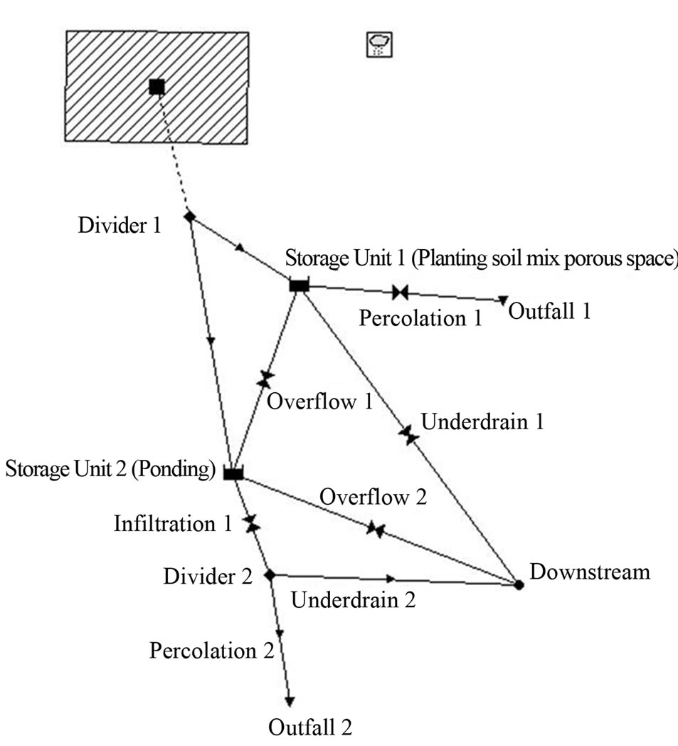
Figure 1. SWMM representation for the bioretention basin (adapted from [25]).
The planting soil mix module is represented with a storage unit (Storage Unit 1), an overflow orifice (Overflow 1), a percolation outlet (Percolation 1), and an underdrain orifice (Underdrain 1). The ponding area module is represented with a storage unit (Storage Unit 2), an overflow orifice (Overflow 2), an orifice that represents ponding water infiltration to the planting soil mix (Infiltration 1), and a flow divider (Divider 2) that separates the infiltrated ponding water between percolation (Percolation 2) and underdrain (Underdrain 2). Percolation to the natural soil is routed to outfall components (Outfalls 1 and 2).
Inflow to the bioretention is first routed to Divider 1, where the flow is separated for infiltration (planting soil mix module) and ponding (ponding area module). The threshold cutoff flow rate (m3/s) for Divider 1 is calculated as the bioretention cell surface area (m2) multiplied by the planting soil mix infiltration rate (m/hr) along with a conversion factor. Flow to the planting soil mix module is first routed to Storage Unit 1, which has an area that is the same as the bioretention surface area with an effective storage depth (heff) equal to the bioretention planting mix soil depth times the porosity. The overflow from Storage Unit 1 is routed to the ponding area module using an orifice representation (Overflow 1). The percolation to the natural soil and drainage via the underdrain system may occur only after the planting soil mix field capacity is exceeded. Percolation is assumed to be at a constant rate and is represented as an outlet (Percolation 1), the rate of which is calculated as the surface area of the bioretention (m2) multiplied by the natural soil infiltration rate (m/hr). The underdrain from the bioretention is represented as an orifice (Underdrain 1). An evaporation factor based on local climate conditions and time of year is assigned to Storage Unit 1 to represent evapotranspiration from the bioretention.
Inflow to the ponding area module is routed to Storage Unit 2, which also has the same area as the bioretention and usually is designed with a maximum depth of 15.2 cm. Overflow from the bioretention ponding area is routed downstream through an orifice (Overflow 2). The ponded water in the ponding area infiltrates into the planting soil mix once water starts leaving the bioretention basin soil through percolation and underdrain. The infiltrated water is routed to a flow divider (Divider 2), where the flow is separated for percolation (Percolation 2) and underdrain. The percolation rate is the same as the percolation rate at Storage Unit 1, and the remaining flow goes through the underdrain (Underdrain 2).
The infiltration from ponding area into the planting soil mix is simulated using an orifice (Infiltration 1). The orifice diameter is calculated based on the orifice flow equation, using the surface area of the bioretention area, planting soil infiltration rate, and the average ponding depth as the input [27].
Infiltration from the ponding area to planting soil mix occurs only after the field capacity is exceeded, and thus a control rule is specified in SWMM to operate the orifice of Infiltration 1. Under the orifice control rule, Infiltration 1 is turned on only when the depth of water in Storage Unit 1 exceeds the equivalent depth of planting soil mix field capacity, hfc, and the orifice is turned off once the depth of water in Storage Unit 1 is below hfc as a result of percolation and underlain drainage.
The representation schemes for porous pavement and green roof are similar to that for the bioretention basin. The difference is that the porous pavement and the green roof do not have a ponding area module. Thus, the representation schemes for the two IMPs do not have the components of Storage Unit 2, Divider 2, Infiltration 1, Overflow 2, Percolation 2, Underdrain 2, and Outfall 2.
2.1.2. Testing of the Representation Schemes
To assess the fidelity of the SWMM representation schemes for bioretention and porous pavement, our proposed representation schemes were tested against the long-term monitoring data from the University of New Hampshire Stormwater Center annual report [26]. The annual report documented long-term average peak flow reduction performances for selected IMPs. The green roof representation scheme was not tested due to a lack of monitoring data.
The hourly rainfall data for the period that matches the UNHSC monitoring duration (01/01/2004-12/31/2006) were obtained from the nearby Rochester Airport, New Hampshire (COOP ID: 277253). The observed annual average evaporation rate from the airport was 0.0023 m/day. Dimensions for the bioretention and porous pavement were obtained from the UNHSC report and were represented accordingly into SWMM, which was run for the three year period. At the end of the simulation, the inflow and outflow hydrographs to each IMP were compiled, and the peak flow reductions were calculated for individual events. The averaged peak flow reduction for bioretention and porous pavement were then compared to the UNHSC report values. The averaged peak flow reduction measures the magnitude of peak flow change between the inflow to, and outflow from, an IMP [28].
A total number of 73 events occurred during 01/01/ 2004 to 12/31/2006, and the SWMM representation for bioretention predicted outflow for 55 events (18 events were fully captured by the bioretention basin). As for the porous pavement representation, the SWMM simulation predicted outflow for 50 events (23 events were fully captured). The average peak flow reductions from the SWMM representations of the two IMPs are compared to the UNHSC observed values, and are summarized in Table 1. As shown in the table, the SWMM representations for bioretention and porous pavement have a satisfactory match of performances to the UNHSC report values.
2.2. Cost of LIDs
The cost of an LID design is the sum of costs for all IMPs used in a particular design. The life-cycle cost of an IMP is composed of the initial construction and material cost and the annual operation and maintenance (O & M) cost. The IMP cost information from the LID Center [29] is used in this study. A summary of the construction cost and the annualized O & M costs for LIDs of bioretention, porous pavement, and green roof is shown in Table 2. As shown, the cost for each LID is a function of the LID surface area, and the annual O & M costs are about five to eight percent of the IMP construction costs. The O & M costs are based on 25-year-life-span assumptions for the IMPs, and the annualized costs include the replacement of LIDs at the 25th year [29]. The land costs and engineering design costs were not included in the cost analysis since they tend to be highly site and project specific [2].
2.3. Hydrologic Model Calibration and Validation
The watershed selected for demonstrating the optimization framework is the Fox Hollow Watershed located in State College, Pennsylvania. The Fox Hollow Watershed, as shown in Figure 2, has an area of 186 hectares and consists of an intensively urbanized Penn State Uni-
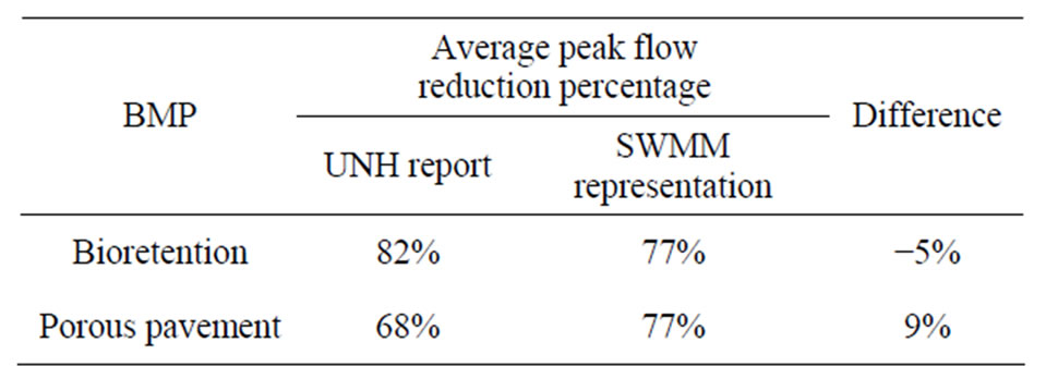
Table 1. Comparison of the long-term SWMM representation predictions and monitored data for IMPs of bioretention and porous pavement.
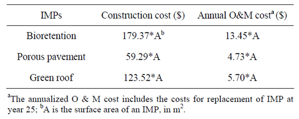
Table 2. Costs for bioretention, porous pavement, and green roof utilized in the optimization analyses (adapted from [28]).
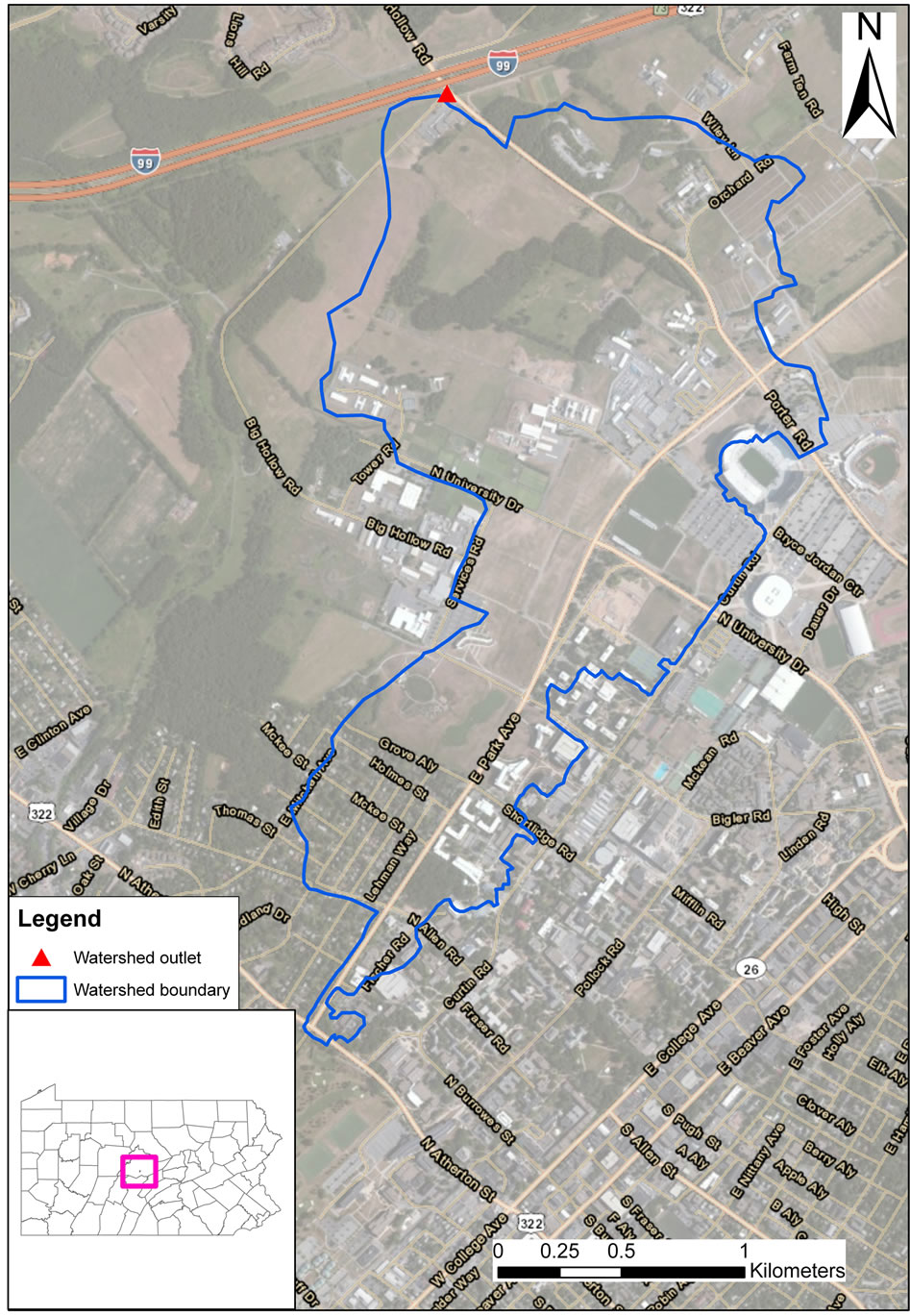
Figure 2. Location of Fox Hollow Watershed in State College, Pennsylvania.
versity campus portion and a less developed meadow/ pasture land portion. In the Borough of State College stormwater regulations (Ordinance 1741, Section 112), postdevelopment peak flow rates should not exceed the pre-development peak flow for 10-year design storms (design return period for sizing stormwater pipes), along with the overall goal of mimicking pre-development runoff conditions. Therefore, our analysis uses the 10-year 24-hour design storm to determine near-optimal tradeoffs between total LID implementation costs and the total runoff volume, while ensuring that the pre-development peak flow rate is not exceeded.
Hydrologic watershed model was calibrated and validated for the Fox Hollow Watershed in preparation for the integrated optimization framework. A SWMM hydrologic model was previously set up for the Fox Hollow Watershed, and the model has been calibrated for several events using data from a nearby 5-minute Penn State University rain gauge (COOP ID: 368449). During the hydrological model calibration, model predictions were compared to the observed hydrograph data recorded at a flow station located near the watershed outlet.
The calibration was conducted through adjusting model parameters of Manning’s n for pervious and impervious surfaces, depression storage for pervious and impervious surfaces, subwatershed width and slope, soil infiltration, and percentages of impervious surfaces with zero depression storage. The model calibration results for a storm that occurred on July 27, 2004 are shown in Figure 3, during which 3.07 cm of rain fell in 10 hours. Through the manual calibration process, the Manning’s n was 0.12 for pervious surfaces and 0.008 for impervious surfaces, the depression storage was 0.86 cm for pervious surfaces and 0.61 cm for impervious surfaces, and the percentage of impervious surfaces with zero depression storage was 4%.
The calibrated model was validated on several independent historical events. Figure 4 shows the validation of model predictions for an event on August 30, 2005, during which 3.23 cm of rain fell in 9 hours. The model appears to perform fairly well in predicting the time to peak and peak flow rate, indicating that the model provides an adequate framework for system-wide hydrologic analysis in the watershed.
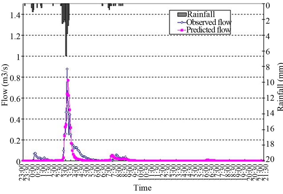
Figure 3. Comparison of the SWMM predicted (after calibration) calibrated and observed flows for the selected event of 07/27/2004 (3.07 cm of rain in 10 hr).
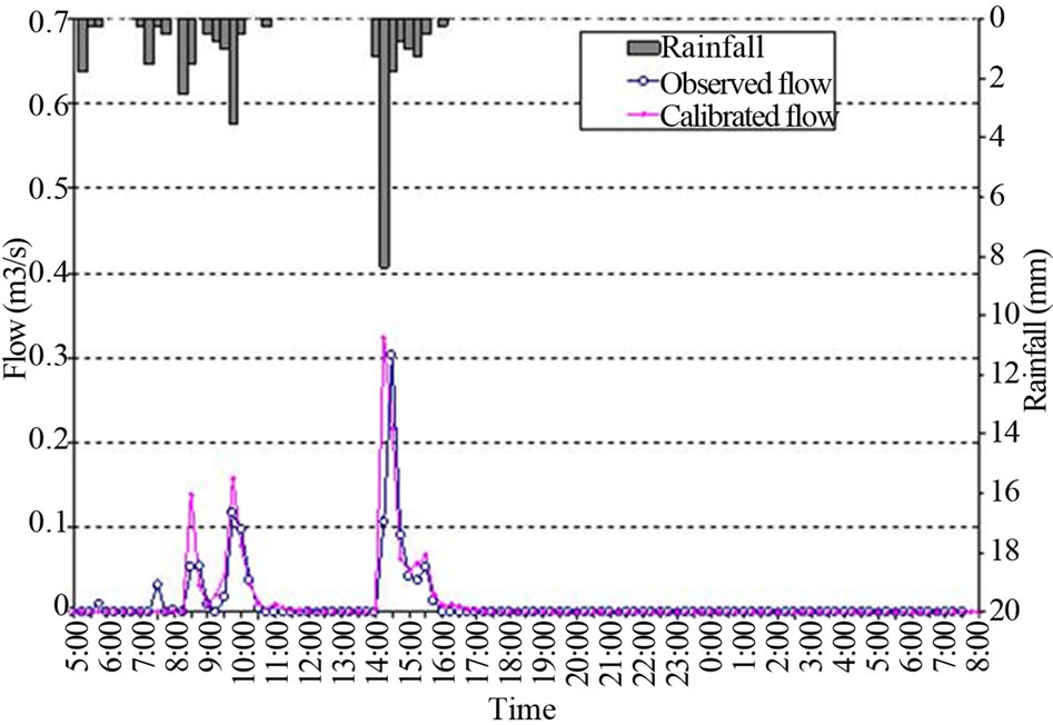
Figure 4. Comparison between observed and SWMM modeled flow for the validation event of 08/30/2005 (3.23 cm of rainfall in 9 hr).
The calibrated hydrologic SWMM model is used to evaluate the existing and future runoff conditions from various design storms. Numerous previous studies have used design storms or single historical storms for optimizing stormwater controls [1,16]. In addition, local stormwater regulations (Ordinance 1741, Section 112, Borough of State College, Pennsylvania) also require that the post-development peak flow rates not exceed the predevelopment peak flow for 10-year design storms (the design return period for existing pipe). For the Fox Hollow Watershed SWMM model, the predicted peak flow rate for the existing conditions is 7.7 m3/s during the 10-year 24-hour design storm.
2.4. LID Design
Each candidate LID design alternative represents a set of IMP implementations in a watershed. In this study, a 17-hectare subwatershed of the less developed portion of the Fox Hollow Watershed is assumed to be developed. In the subwatershed, six buildings, two parking lots, and associated sidewalks are assumed to be implemented, and the LID practices are then applied to the post-development subwatershed. In setting up the LID analysis, all the rooftops (up to 90% of the total roof area, assumeing 10% of the roof area for ventilation facilities) are available for green roof implementation, and all the parking lots are available for porous pavement implementation. In addition, four bioretention areas located adjacent to the buildings and parking areas are also available for implementation. The locations of the thirteen LIDs are shown in Figure 5.
The bioretention is designed to have a 0.15 m depth of ponding area and a 0.76 m depth of planting soil mix, underlain with 0.30 m of gravel layer. Porosity for both the planting soil mix and the gravel layer is chosen to be
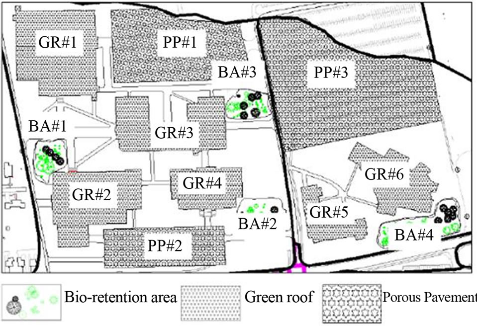
Figure 5. The LID design site layout showing the 13 locations for the IMPs of bioretention area, green roof, and porous pavement for the selected subwatershed of the Fox Hollow Watershed.
40%. The infiltration rate for the planting soil is 0.10 m/hr, and the infiltration rate for the gravel layer is 0.36 m/hr. The porous pavement is designed to have a 0.10 m layer of porous asphalt, a 0.1 m layer of chocker course, a 0.61 m layer of sand filter, and a 0.20 m layer of gravel. Porosities for the four layers are 15%, 25%, 25%, and 35%, and infiltration rates are 19.05 m/hr, 0.36 m/hr, 0.36 m/hr, and 0.36 m/hr, respectively. The green roof is designed to have a 0.12 m depth of growth medium, with a porosity of 35% and an infiltration rate of 0.52 m/hr.
When implementing the IMPs in proposed locations within the Fox Hollow Watershed, ratios of the IMP areas to the total subwatershed area are used to represent IMP sizes, rather than using the real IMP area values. The percentage-based representation of IMPs implicitly ensures that the boundaries of proposed areas of LID application are satisfied and do not require specialized constraints when using evolutionary multi-objective search. The percentages of the six green roofs vary from zero to 90% for the six corresponding rooftop areas. The percentages of areas of the three porous pavements vary from zero to 100% of the corresponding parking lot areas. Percentages of the four bio-retention areas vary from zero to 100% of the maximum areas allowed at the four corresponding site locations. Area changes of all IMPs are set at a 10% interval (i.e. 0%, 10%, 20%, etc.) when the optimization algorithm is implemented. The maximum areas of these IMPs are shown in Table 3.
With IMP areas being represented with ratios of the maximum areas allowed, a string of thirteen real numbers between 0 and 1 characterizes a possible LID design alternative in the watershed. A one-to-one projection is established between the numbers in the string and the IMPs on the ground. Each LID design alternative string is divided into three sections for representing the IMPs in the order of porous pavement, green roof, and the bioretention area. The first three entries in the string represent the percentages of porous pavement implementations on parking lots #1, #2, and #3, respectively. The next six entries are the percentages of green roof implementations
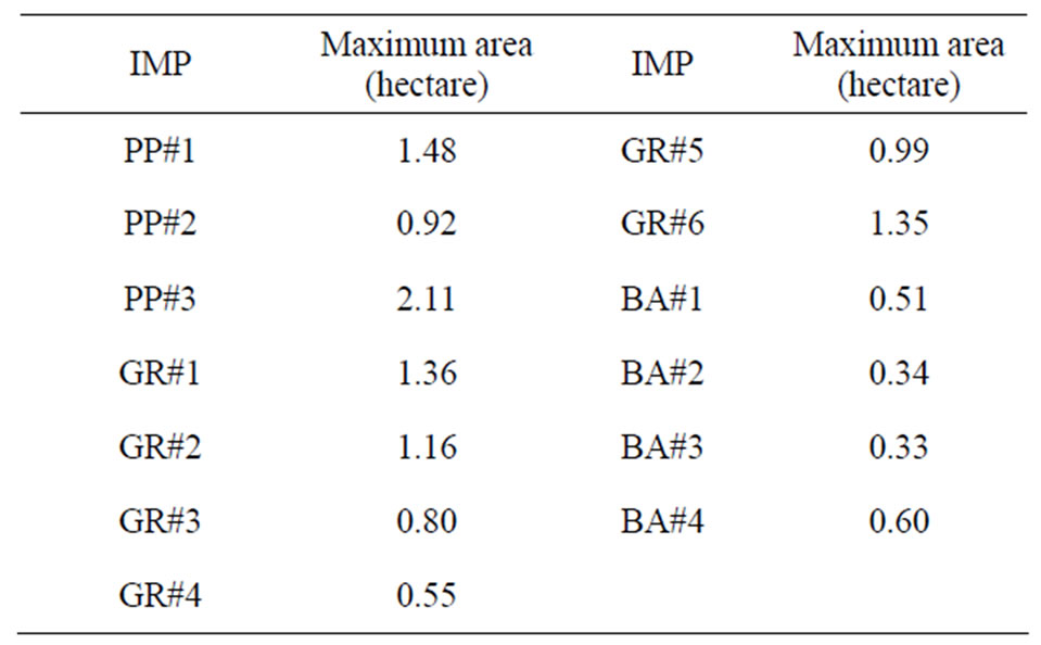
Table 3. Maximum areas of IMPs in the LID design.
on rooftops #1 to #6, and the last four entries are the percentages of bioretention surface areas to the maximum areas allowed at the locations BA#1 to BA#4. Figure 6 shows a sample string representation of IMPs based on this approach, wherein the first 3 cells represent the ratios for porous pavement at the four parking lots, the next 6 cells represent the ratios for green roofs, and the last 4 cells represent the ratios of bioretention areas.
2.5. Optimization Model
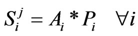
Optimization of urban stormwater management is the process of identifying tradeoffs between conflicting goals such as maximizing stormwater control while minimizing the total cost. Given a watershed with m possible locations for IMP implementations and n IMP types that can be selected for building LID designs, the optimization of LID designs in meeting peak flow control requirements can be stated as:
Objectives:
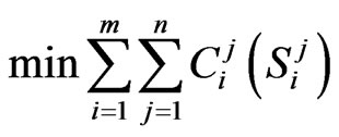 (1)
(1)
 (2)
(2)
Subject to:
 (3)
(3)
 (4)
(4)
 (5)
(5)
 (6)
(6)
where  = cost of IMP type j at location i,
  = the size of IMP type j at location i, VLID = total runoff volume from the LID design, QpLID = peak flow rate from the LID design, Qppre = pre-development watershed peak flow rate, Si = feasible range of IMP sizes at location i, Ai = maximum area allowed for IMP implementation at location i, pi = percentage of IMP implementation to the maximum area allowed at location i, m = total number of possible locations to apply IMP techniques, and n = total number of available IMP techniques.
2.6. NSGAII and ε-NSGAII
The genetic algorithm (GA) is based upon the theory of natural selection and genetic propagation, in which the stochastic technique maintains a population of solutions
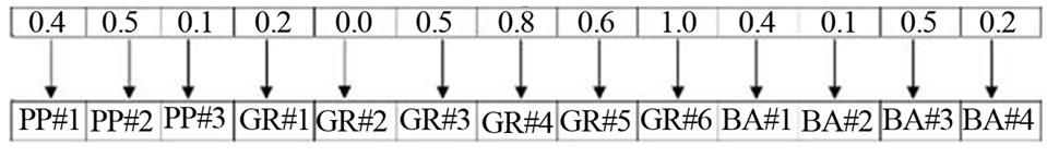
Figure 6. Sample string indicating the ratio of IMP area to total area for an individual LID design used during the optimization process.
and evolves to create more efficient generations [30]. Genetic algorithms are one of the most commonly used techniques for optimizing stormwater management [17]. Genetic algorithms are often used for challenging problems such as stormwater management since they are able to approximate optimal solutions for discrete, non-convex, and highly nonlinear decision spaces [1].
The non-dominated Sorted Genetic Algorithm-II (NSGAII) developed by Deb, et al. [31] is a revision from the original Non-dominated Sorted Genetic Algorithm (NSGA) [32]. Compared to the original version, NSGAII reduced the computational complexity, incurporated explicit elitism, and eliminated the need for specifying the sharing parameter of σ share [33]. In NSGAII, a solution is ranked according to the number of solutions that dominate it. A two-step crowded binary tournament selection is then carried out based on the fitness value of each solution. During the process, the solution with a lower fitness rank is always preferred. When two solutions have the same rank, the one with a larger crowding distance is selected. By doing this, NSGAII ensures a more distributed set of solutions along the final Pareto front [34].
This study employs a further revision of NSGAII termed the ε-NSGAII, which adds ε-dominance archiving, adaptive population sizing, and automatic termination to the original NSGAII algorithm [34]. The use of ε-dominance archiving allows the user to specify how precisely each solution is evaluated while promoting diverse representations of tradeoffs [35]. A large ε value means a coarser grid of the solution space (which means less ultimate solutions) and vice versa. After a user-specified number of generations within each run, the ε-NSGAII algorithm automatically adapts its population size according to the “archived” best solutions ever found. Using an injection scheme, the adapted population consists of 25% of the ε-non-dominated archive solutions and 75% of new randomly-generated solutions. The ε- NSGAII algorithm has been successfully applied to a wide range of problems, in which the algorithm has demonstrated significant advantage over the NSGAII algorithm in both the time to converge and the diversity of solutions [36-38].
When using the ε-NSGAII algorithm, the user needs to specify an initial population size from which the algorithm starts. Other required parameters include the maximum number of function evaluations (nfe) and the maximum generations per run.
2.7. Optimization Framework Setup
2.7.1. Optimization Algorithm
The optimization framework builds the SWMM model as a subroutine of the ε-NSGAII algorithm. Both ε-NSGAII and SWMM are available in C code, and a string of numbers representing IMP sizes can be generated by ε-NSGAII and passed onto SWMM for evaluation. The SWMM simulated results can then be sent back to ε- NSGAII for evaluation against objectives of total cost and runoff volume and the constraint of peak flow rate. An overview of the optimization process is shown in Figure 7.
As shown, the ε-NSGAII algorithm reads the SWMM model input in the beginning, and then uses a two-tier loop structure to carry out the optimization process. The outside loop uses the maximum number of function evaluations (nfe) supplied by the user as the stopping criteria. At the beginning of the outside loop, an initial population (N) of LID designs is randomly generated. Each individual in the population is a string of real numbers that represent a coded LID design. Each number in the string corresponds to the size of a specific IMP in the LID design (sample representation presented in Figure 6). After the first generation of LID designs is generated, the SWMM model sub-routine is called to estimate the peak flow rate and total runoff volume from each LID design in the population. Meanwhile, the total cost of each LID design is calculated using the cost function (as shown in Table 1) for each IMP in the design. The peak flow rate from each LID is compared to the pre-development watershed peak flow. If the LID design peak flow rate is larger than the pre-development peak flow

Figure 7. The LID optimization framework utilizing the SWMM model for evaluating hydrologic response for generated designs.
rate, then the LID design is penalized by adding 1012 to both the total runoff volume and total cost. The LID designs are then ranked in the ε-NSGAII algorithm using a fast ε-non-dominant sorting strategy [31]. Since the optimization process is to minimize the total cost and total runoff volume from the watershed, the penalized LID designs are ranked last during the sorting. The mutation and crossover operators are then applied to the LID individuals to create a child population.
The run time for calculations in the inside loop is decided by another user-supplied parameter, the maximum number of generations per run. At the beginning of the inside loop, the parent and child populations from the outside loop are combined. The combined population (2N) of LID designs is sent to the SWMM model for peak flow and total runoff volume estimations. Meanwhile, the cost of each LID design is calculated by adding the cost of each IMP in the LID design. The peak flow rate from each LID design is compared to the pre-development watershed peak flow rate. The LID designs with a peak flow rate larger than the pre-development watershed peak flow rate are penalized by adding 1012 to the total cost and total runoff volume, respectively. The ε-non-dominant sorting is then applied to the combined population of LID individuals, and the best solutions are stored in an offline archive. The first N LID designs in the sorted 2N population then become the updated parent population. Tournament selection, simulated binary crossover and polynomial mutation are then applied to the updated parent population, and a new child population (N) is created. The child and parent populations are then combined and a new loop begins. After the maximum number of generations per run is reached, the inside loop stops and the population size (N) is updated with reference to the size of best solutions archive. If M best LID designs are kept in the archive, then 3M more LID designs are generated randomly and combined with the M existing solutions. Thus, a new population size of 4M is used to replace the former population size of N. This population injection approach is used by the ε- NSGAII algorithm not only to preserve the best solutions ever found but also to introduce diversity into the solution population [30].
The LID optimization process finishes when the maximum number of function evaluations (nfe), as specified by the user, is reached. At the end of the optimization process, the solutions retained in the archive of best solutions are the non-dominated Pareto-front of LID designs.
2.7.2. Parameters for Optimization Setup
The optimization framework parameters include the initial population size, maximum population size, maximum generations per run, maximum number of function evaluations, probability for crossover, and probability for mutation. The parameter settings for the optimization framework in this study are shown in Table 4.
3. Results and Discussion
The 10-year 24-hour design storm is used to run the SWMM model in the LID optimization framework. The pre-development peak flow rate is used as the constraint during the optimization process, and LID designs with a peak flow rate larger than the pre-development peak flow rate (7.7 m3/s) are penalized. The optimization process takes about 23 hours on an Intel Quad Core CPU Q9400 2.66 GHz processor and 3.0 GB random access memory (RAM). Figure 8 shows all the possible solutions (excluding 1222 penalized solutions that had peak flow rate larger than 7.7 m3/s), along with 37 near-optimal solutions identified by ε-NSGAII.
As shown in Figure 8, the 37 near-optimal LID designs define an approximation to the Pareto front between the total LID design cost and the total runoff volume. The tradeoff curve shows that as the total cost increases, the total runoff volume from the watershed gen-
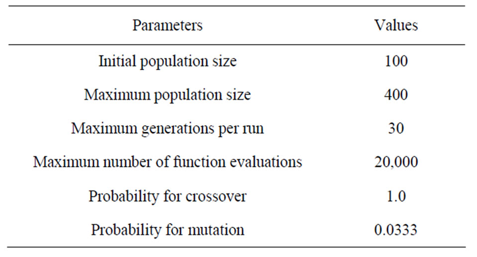
Table 4. Parameter settings for the LID optimization framework.
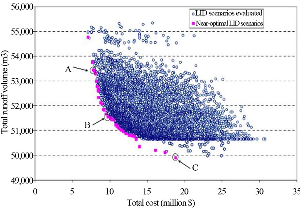
Figure 8. The tradeoff between the LID design total cost and total runoff volume for the 10-year 24-hour design event in the FHW, along with three scenarios (A, B, and C) for further hydrologic analysis.
erally decreases, and vice versa. In addition, as the total LID design cost increases, the marginal rate of return in total runoff volume reduction decreases. For example, for three near-optimal solutions A, B, and C noted in Figure 8, the total cost increase from solution A to solution B is $2.32 million, and the runoff volume decrease is 1,929 m3. As the solution switches from B to C, however, the total cost increase is $8.68 million, and the runoff volume decrease is only 1619 m3. Figure 8 also shows that at a certain level of treatment (total runoff volume) the corresponding LID design can vary quite significantly. For example, when the total runoff volume is 50,629 m3, the total cost of LID scenario may range from $13.54 million to $30.73 million. This demonstrates the benefit of the optimization framework, through which a wide range of possible designs are evaluated and the most cost-effective alternatives are identified.
The total runoff volume and total cost of the 37 nearoptimal designs are shown in Table 5 through Table 7, in which the total LID scenario cost, corresponding total runoff volume, and the area percentages for porous pavement, green roof, and bioretention are listed. The LID designs in the tables are ranked in the descending order of total cost. As shown in the tables, a higher total LID scenario cost corresponds to higher area percentages of the three IMPs and lower total runoff volume. As the total LID scenario cost decreases from near optimal solution #1 through solution #37, the area percentages of all the three IMPs in general also decreases. In addition, larger area percentages of bioretention are more frequently selected to form LID the near-optimal LID scenarios than those of the porous pavement and green roof IMPs.
The relatively more frequent selection of the bioretention area can be explained by the locations of the bioretention areas. All the four bio-retention areas are designed to detain and infiltrate the surface runoff from surrounding areas, whereas the green roof and porous pavement are designed to reduce surface runoff at a particular site (i.e. rooftop or parking lot). When comparing the effects on runoff conditions, the effects of the bioretention area are more “regional” and the effects of green roof and the porous pavement are more “local”. The optimization process searches for the cost-effective stormwater management practices, and the relatively larger hydrological benefits provided by the bioretention areas make them preferred despite their higher unit cost. The reason that bioretention area #1 and #2 tend be selected with higher percentages is similar. Among the four bioretention areas, bioretention #1 treats runoff from the neighboring College Height area (to the west of BA#1) and bioretention #2 treats runoff from GR#1 to #4, PP#1 and #2, and BR#1 and #3. In comparison, bioretention areas #3 and #4 are more “localized” and treat smaller
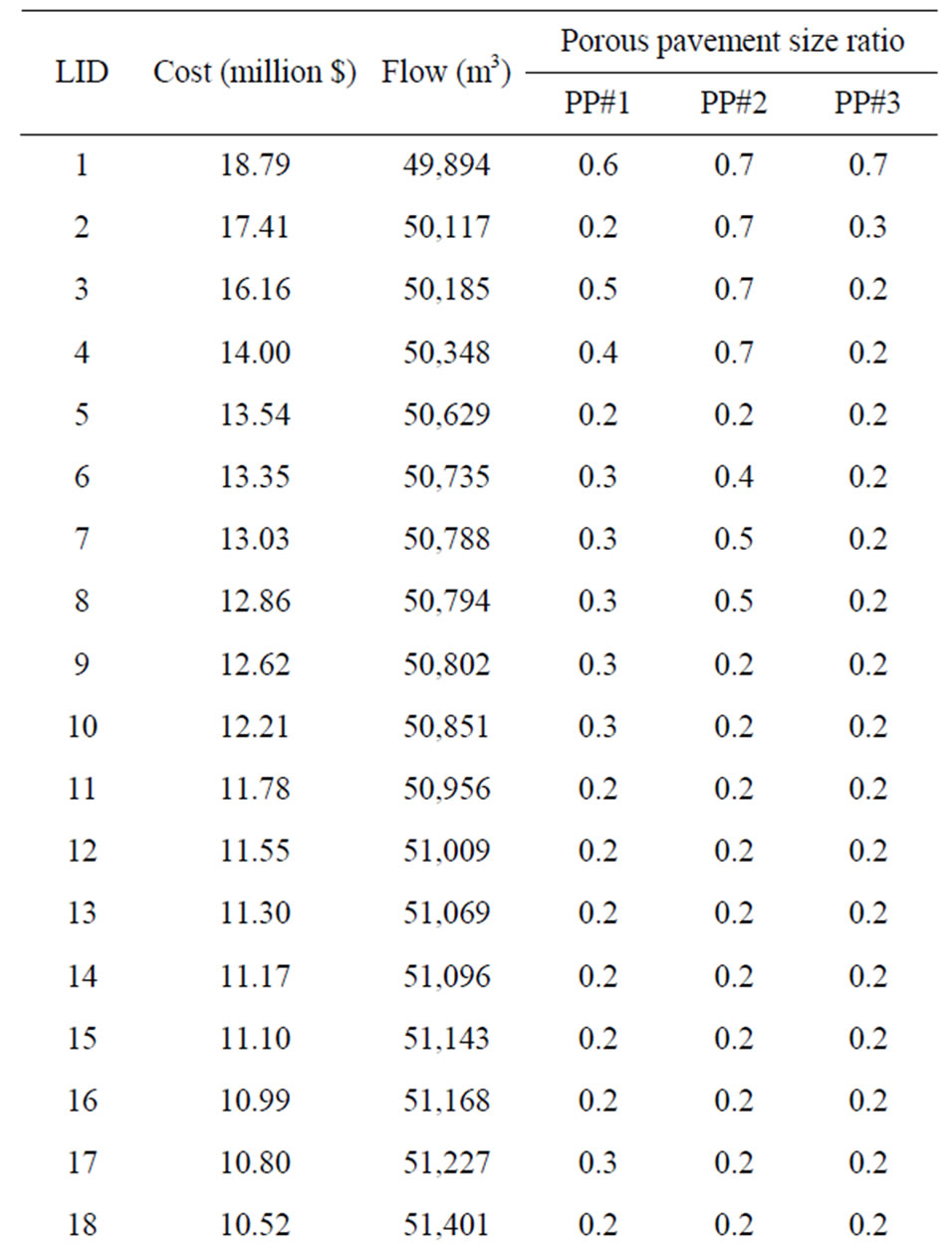
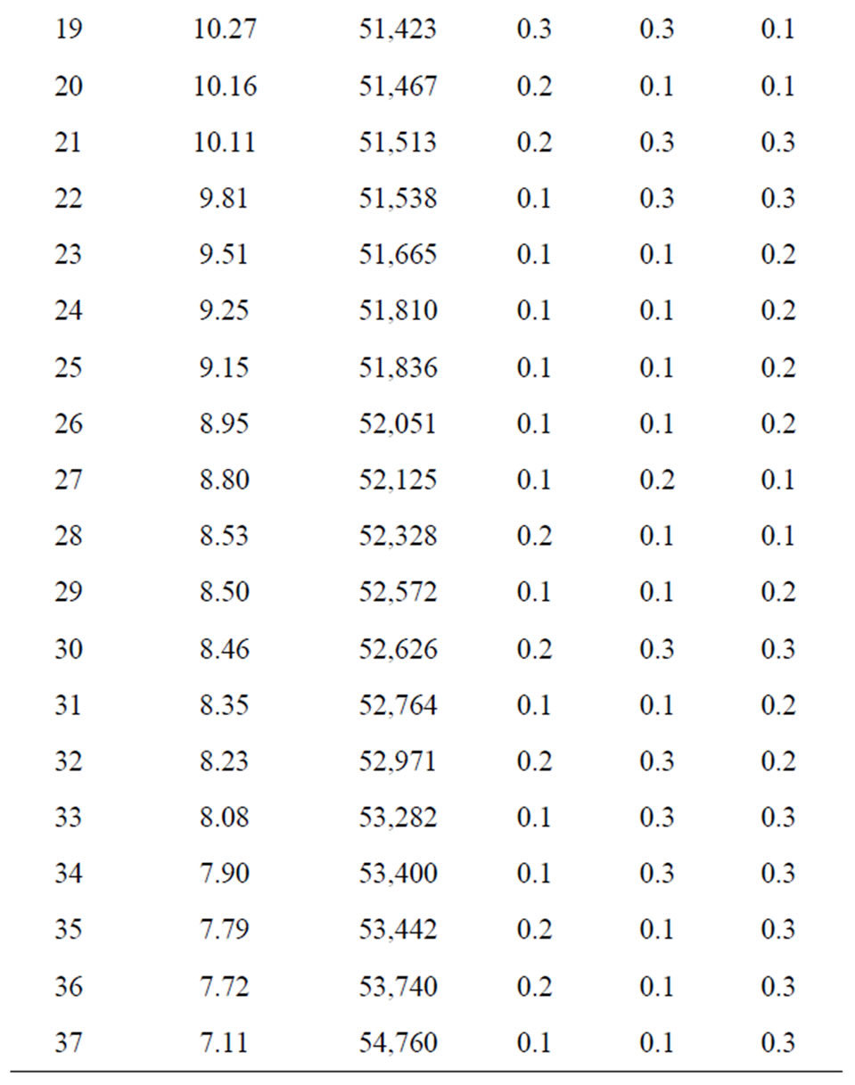
Table 5. Near-optimal porous pavement sizing ratios in optimal LID designs identified by the optimization framework.
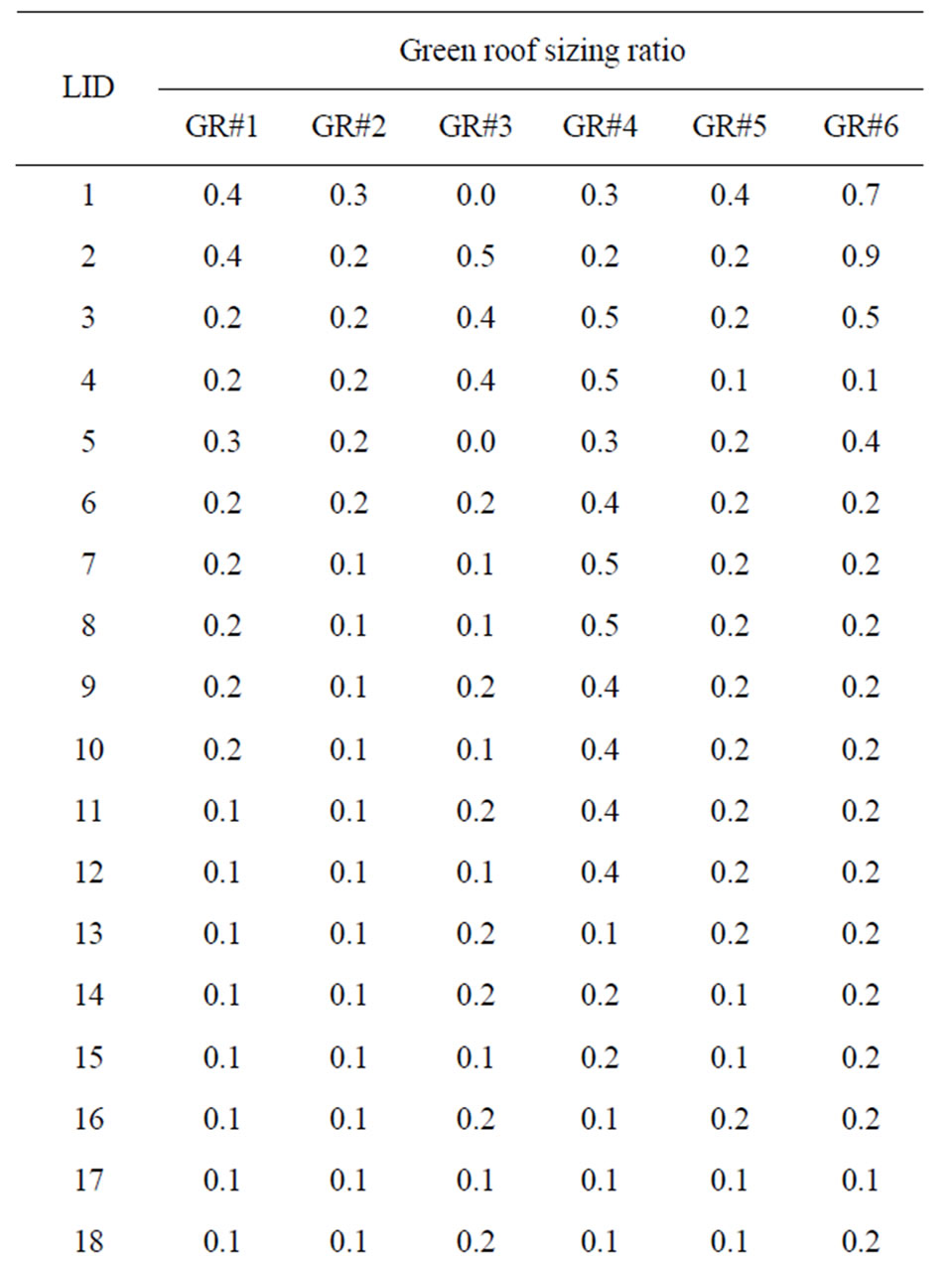
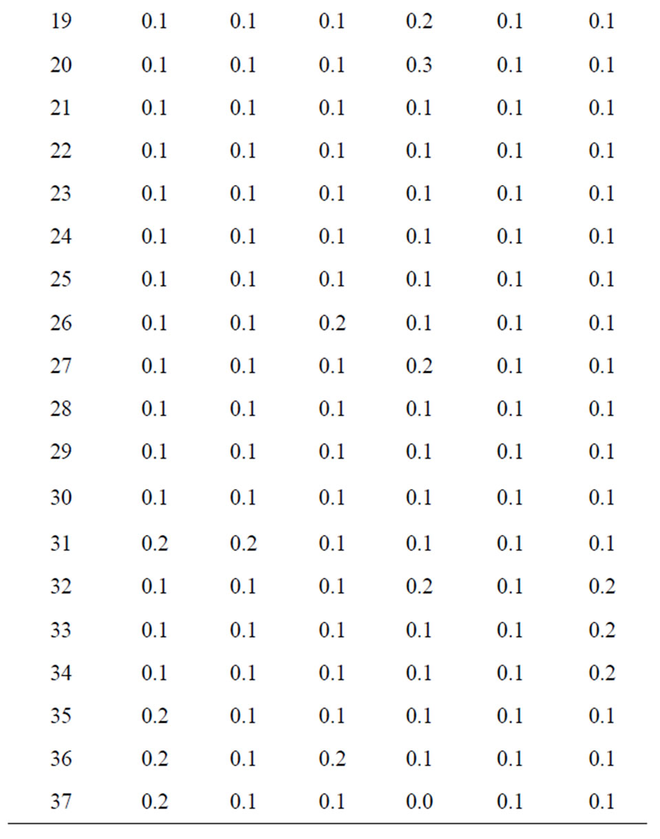
Table 6. Near-optimal green roof sizing ratios in LID designs identified by the optimization framework.
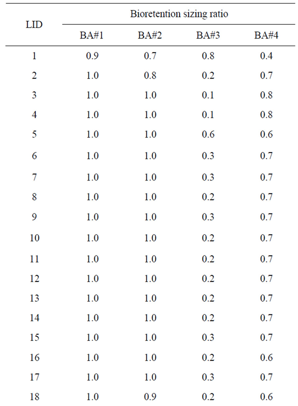
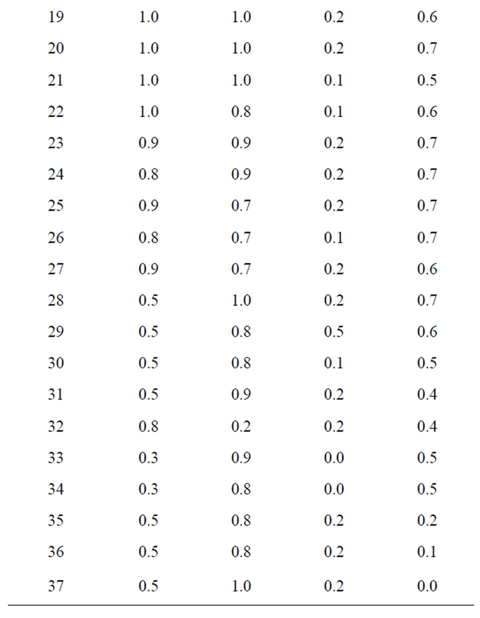
Table 7. Near-optimal bioretention sizing ratios in LID designs identified by the optimization framework.
areas as compared to bioretention areas #1 and #2. This demonstrates how the spatial locations of the IMPs could impact the optimization results, and also highlights the importance of having a distributed model such as SWMM to conduct the simulation.
Runoff conditions from the three near-optimal LID scenarios in Figure 8 are illustrated in Figure 9. The LID scenarios A, B, and C are solutions #35, #21, and #1 in Table 5, respectively. The LID cost increases from Scenario A to B to C. The figure shows a seven-hour span of the runoff hydrograph for the 24-hour design event to highlight the runoff rates for the different scenarios. As shown, the peak flow rate from the lowest cost LID scenario of the three (Scenario A) is close to (difference = 0.06 m3/s, or 0.7%) the pre-development peak flow rate. A more expensive LID scenario helps further reduce the peak flow rate from the watershed. The peak flow difference between LID Scenario C and the predevelopment peak flow rate is 0.8 m3/s, or 11%. Figure 9 also shows the increase in total runoff volume as the total LID cost decreases. As compared to the pre-development watershed runoff volume, the total runoff volume increases by 5%, 2%, and 1% for Scenarios A, B, and C, respectively. The more expensive LID scenarios have larger IMPs and thus can provide more infiltration, which eventually leads to increased groundwater recharge and sustained base flow.
The developed optimization framework can be expanded for optimizing different LID implementation designs. The relatively independent relationship between ε-NSGAII and SWMM allows for more IMPs and at different locations within a watershed, which can be updated in SWMM and then sent back to ε-NSGAII. With the SWMM capability for continuous simulations, the optimization framework can also optimize LID designs with respect to long-term performances.
The new watershed management framework carries out optimization analysis on LID scenarios that consist of
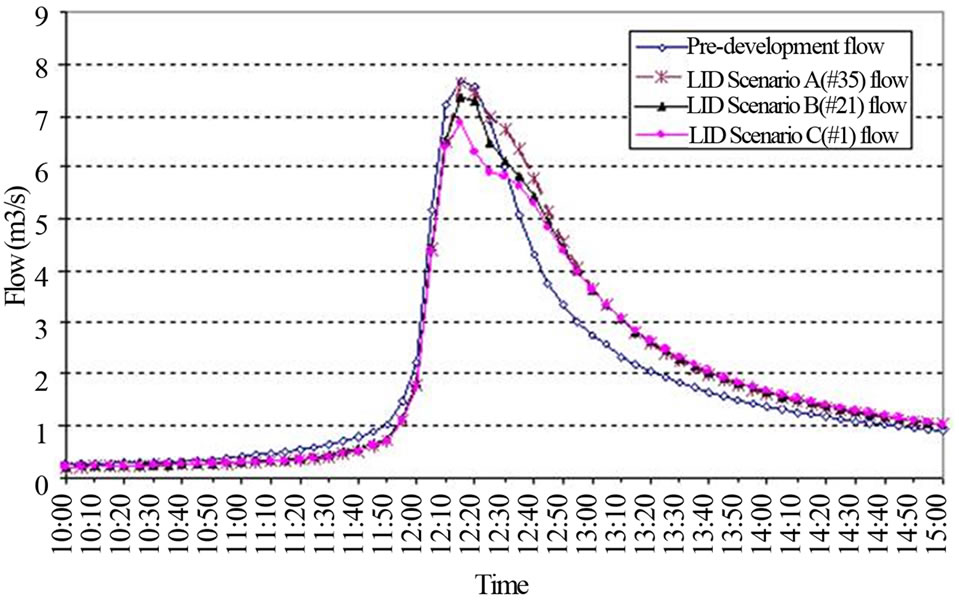
Figure 9. Runoff conditions from three near-optimal LID scenarios as compared to the pre-development watershed runoff.
three different types of IMPs simultaneously. This is an improvement from previous studies in which only one single type of IMP is investigated [1,17]. Due to variances in hydrologic benefits provided by each type of IMP, the optimization framework is able to have a more comprehensive evaluation of possible LID designs. The developed optimization framework also accounts for non-linear hydrologic processes in an IMP. The physiccally-based LID representation can account for hydrologic processes including infiltration, percolation, evapotranspiration, and ponding. These features help improve the performance evaluation of the LID design as compared to simplified IMP representation schemes (e.g. CN method in [1]), especially for long-term simulations.
The developed optimization framework enables distributed representation of IMPs, and their effects on hydrologic routing are accounted for through the SWMM model. The placement and sizing of IMPs influences the timing and magnitude of downstream hydrographs due to convolution. This echoes conclusions from previous studies that demonstrate the necessity of a distributed watershed model when describing the complicated spatial and temporal relationships between land simulation and watershed peak flow reduction [1,17,39].
The optimization framework could be expanded to optimize on water quality objectives as well. Ongoing efforts are underway to develop water quality models for the FHW. After the water quality model is calibrated and verified, the water quality predictions of the SWMM model can be used for optimization objectives. In order to accommodate water quality related optimizations, a long-term simulation would be necessary and the optimization target will be the reduction of pollutant load between the post-development and the pre-development conditions. The ε-NSGAII algorithm, meanwhile, can be readily adjusted to include water quality pollutants as an additional optimization objective.
4. Summary and Conclusion
Representation schemes for LID techniques in the distributed SWMM model are presented, and the schemes are then linked with the ε-NSGAII algorithm to build a multi-objective optimization framework for peak flow management in an urbanizing watershed. The optimization framework identifies 37 LID scenarios that form the near-optimal Pareto frontier, which shows diminishing marginal benefits in peak flow reduction as the total cost increases. Optimization results using this multi-objective optimization approach linked with SWMM can help municipalities and watershed authorities make informed decisions regarding possible selection and location of various IMPs to be considered in stormwater management.
The optimization results indicate that the spatial location of IMPs can influence the compositions of the nearoptimal LID scenarios identified. In the case study, the bioretention area is selected more frequently and with larger sizes at two sites, even though the bioretention area is a relatively more expensive practice. The main reason is that the bioretention area treats runoff from surrounding areas at those two places, and thus has a regional impact on the hydrologic benefits provided. The distributed structure of the SWMM model allows for the representation and evaluation of such impacts among IMPs during the optimization process. At the same time, the generic structure of the optimization framework also makes it possible to flexibly evaluate various IMP implementation scenarios in a watershed.
5. Acknowledgements
The authors appreciate the help from Dr. Robert Roseen formerly at the University of New Hampshire Stormwater Center. This project was jointly funded by the Department of Agricultural and Biological Engineering and the Office of Physical Plant at the Penn State University. The authors also thank the anonymous reviewers for their constructive comments that helped improve this paper.
REFERENCES
- C. Perez-Pedini, J. F. Limbrunner and R. M. Vogel, “Optimal Location of Infiltration-Based Best Management Practices for Storm Water Management,” Journal of Water Resources Planning and Management, Vol. 131, No. 6, 2005, pp. 441-448. http://dx.doi.org/10.1061/(ASCE)0733-9496(2005)131:6(441)
- D. J. Sample, J. P. Heaney, L. T. Wright and R. Kuostats, “Geographic Information Systems, Decision Support Systems, and Urban Storm-Water Management,” Journal of Water Resources Planning and Management, Vol. 127, No. 3, 2001, pp. 155-161. http://dx.doi.org/10.1061/(ASCE)0733-9496(2001)127:3(155)
- Prince George’s County, “Low Impact Development Design Strategies: An Integrated Design Approach,” Department of Environmental Resources Programs and Planning Division, Largo, 1999.
- A. H. Elliott and S. A. Trowsdale, “A Review of Models for Low Impact Urban Stormwater Drainage,” Environmental Modeling & Software, Vol. 22, No. 3, 2007, pp. 394-405. http://dx.doi.org/10.1016/j.envsoft.2005.12.005
- M. Dietz, “Low Impact Development Practices: A Review of Current Research and Recommendations for Future Directions,” Water, Air, & Pollution, Vol. 186, No. 4, 2007, pp. 351-363. http://dx.doi.org/10.1007/s11270-007-9484-z
- US Environmental Protection Agency (USEPA), “Low Impact Development: A Literature Review,” Office of Water, Washington DC, 2000.
- Puget Sound Action Team (PSAT), “Low Impact Development: Technical Guidance Manual for Puget Sound,” Puget Sound Action Team (PSAT), Olympia, 2005.
- Pennsylvania Department of Environmental Protection (PADEP), “Pennsylvania Stormwater Best Management Practices Manual,” Bureau of Watershed Management, PADEP, Harrisburg, 2006.
- Massachusetts Department of Environmental Protection (MassDEP), “Massachusetts Stormwater Handbook,” Massachusetts Department of Environmental Protection, Worcester, 2008.
- D. Ackerman and E. D. Stein, “Evaluating the Effectiveness of Best Management Practices Using Dynamic Modeling,” Journal of Environmental Engineering, Vol. 134, No. 8, 2008, pp. 628-639. http://dx.doi.org/10.1061/(ASCE)0733-9372(2008)134:8(628)
- Center for Watershed Protection (CWP), “National Pollutant Removal Performance Database, Version 3,” Center for Watershed Protection (CWP), Ellicott City, 2007.
- J. Clary, J. Jones, E. Strecker and M. Quigley, “International Stormwater BMP Database: What’s in It for You?” Proceedings World and Environmental Water Resources Congress, Sustainability from the Mountains to the Sea, Honolulu, 12-16 May 2008, pp. 1-10.
- S. Cryer, M. Fouch, A. Peacock and P. Havens, “Characterizing Agrochemical Patterns and Effective BMPs for Surface Waters Using Mechanistic Modeling and GIS,” Environmental Modeling & Assessment, Vol. 6, No. 3, 2001, pp. 195-208. http://dx.doi.org/10.1023/A:1011978420760
- W. F. Coon, “Simulating Land-Use Changes and Stormwater Detention Basins and Evaluating Their Effect on Peak Stream Flows and Stream Water Quality in Irondequoit Creek Basin, New York—A User’s Manual for HSPF and GenScn,” Open-File Rep. 03-136, US Geological Survey, Reston, 2003.
- W. Heasom, A. Welker and R. Traver, “Hydrologic Modeling of a Bioinfiltration Best Management Practice,” The Journal of the American Water Resources Association, Vol. 42, No. 5, 2006, pp. 1329-1347. http://dx.doi.org/10.1111/j.1752-1688.2006.tb05616.x
- L. J. Harrell and S. R. Ranjithan, “Detention Pond Design and Land Use Planning for Watershed Management,” Journal of Water Resources Planning and Management, Vol. 129, No. 2, 2003, pp. 98-106. http://dx.doi.org/10.1061/(ASCE)0733-9496(2003)129:2(98)
- X. Zhen, S. L. Yu and J. Lin, “Optimal Location and Sizing of Stormwater Basins at Watershed Scale,” Journal of Water Resources Planning and Management, Vol. 130, No. 4, 2004, pp. 339-347. http://dx.doi.org/10.1061/(ASCE)0733-9496(2004)130:4(339)
- J. P. Heaney and L. T. Wright, “Integrating Statistical Methods and Continuous Simulation for Evaluating Urban Stormwater Systems,” In: W. James, Ed., Stormwater and Water Quality Management Modeling, CHI Press, Guelph, 1997, pp. 45-76.
- M. W. Gitau, T. L. Veith, W. J. Bgurek and A. R. Jarrett, “Watershed Level Best Management Practice Selection and Placement in the Town Brook Watershed, New York,” Journal of The American Water Resources Association, Vol. 42, No. 6, 2006, pp. 1565-1581. http://dx.doi.org/10.1111/j.1752-1688.2006.tb06021.x
- C. Maringanti, I. Chaubey and J. Popp, “Development of a Multiobjective Optimization Tool for the Selection and Placement of Best Management Practices for Nonpoint Source Pollution Control,” Water Resources Research, Vol. 45, No. 6, 2009, Article ID: W06406. http://dx.doi.org/10.1029/2008WR007094
- M. Cheng, J. X. Zhen and L. Shoemaker, “BMP Decision Support System for Evaluating Stormwater Management Alternatives,” Frontiers of Environmental Science & Engineering in China, Vol. 3, No. 4, 2009, pp. 453-463. http://dx.doi.org/10.1007/s11783-009-0153-x
- US Environmental Protection Agency (USEPA), “SUSTAIN-A Framework for Placement of Best Management Practices in Urban Watersheds to Protect Water Quality,” Office of Water, Washington DC, 2009.
- M. Cheng, J. X. Zhen and L. Shoemaker, “BMP Decision Support System for Evaluating Stormwater Management Alternatives,” Frontiers of Environmental Science & Engineering in China, Vol. 3, No. 4, 2009, pp. 453-463. http://dx.doi.org/10.1007/s11783-009-0153-x
- J. G. Lee, A. Selvakumar, K. Alvi, J. Riverson, J. X. Zhen, L. Shoemaker and F. Lai, “A Watershed-Scale Design Optimization Model for Stormwater Best Management Practices,” Environmental Modeling & Software, Vol. 37, 2012, pp. 6-18. http://dx.doi.org/10.1016/j.envsoft.2012.04.011
- L. A. Rossman, “Stormwater Management Model User’s Manual: Version 5.0. EPA/600/R-05/040,” National Risk Management Research Laboratory, Office of Research and Development, USEPA, Cincinnati, 2005.
- S. Guitierrez, “US EPA’s Urban Watershed Research Program in BMPs and Restoration for Water Quality Improvement,” In: S. Struck, A. Tafuir and M. Ports, Eds., BMP Technology in Urban Watersheds: Current and Future Directions, ASCE Publications, 2006, pp. 1-17.
- G. Zhang, J. M. Hamlett and T. Saravanapavan, “Representation of Low Impact Development Designs in SWMM,” In: W. James, K. Irvine, J. Li, E. McBean, R. Pitt and S. Wright, Eds., Dynamic Modeling of Urban Water Systems, CHI Press, Guelph, 2009, pp. 183-198.
- University of New Hampshire Stormwater Center (UNHSC), “2007 Annual Report,” UNHSC, Durham, 2007.
- Low Impact Development Center (LID Center), “Low Impact Development for Big Box Retailers,” Prepared under EPA Assistance Agreement #AW-83203101, Beltsville, 2005.
- D. E. Goldberg, “Genetic Algorithms in Search, Optimization, and Machine Learning,” Addison-Wesley, Reading, 1989.
- K. Deb, A. Pratap, S. Agarwal and T. Meyarivan, “A Fast and Elitist Multiobjective Genetic Algorithm: NSGAII,” IEEE Transactions on Evolutionary Computation, Vol. 6, No. 2, 2002, pp. 182-197. http://dx.doi.org/10.1109/4235.996017
- K. Deb and R. B. Agrawal, “Simulated Binary Crossover for Continuous Search Space,” Complex Systems, Vol. 9, No. 2, 1995, pp. 115-148.
- C. A. Coello Coello, D. A. Van Veldhuizen and G. B. Lamont, “Evolutionary Algorithms for Solving Multi-Objective Problems,” Kluwer Academic Publishers, New York, 2002. http://dx.doi.org/10.1007/978-1-4757-5184-0
- J. B. Kollat and P. M. Reed, “Comparing State-of-the-Art Evolutionary Multi-Objective Algorithms for Long-Term Groundwater Monitoring Design,” Advances in Water Resources, Vol. 29, No. 6, 2006, pp. 792-807. http://dx.doi.org/10.1016/j.advwatres.2005.07.010
- J. B. Kollat and P. M. Reed, “A Computational Scaling Analysis of Multiobjective Evolutionary Algorithms in Long-Term Groundwater Monitoring Applications,” Advances in Water Resources, Vol. 30, No. 3, 2007, pp. 408-419. http://dx.doi.org/10.1016/j.advwatres.2006.05.009
- Y. Tang, P. M. Reed and T. Wagener, “How Effective and Efficient Are Multiobjective Evolutionary Algorithms at Hydrologic Model Calibration?” Hydrology and Earth System Science, Vol. 10, No. 2, 2006, pp. 289-307. http://dx.doi.org/10.5194/hess-10-289-2006
- Z. Zhang, T. Wagener, P. M. Reed and R. Bhushan, “Reducing Uncertainty in Predictions in Ungauged Basins by Combining Hydrologic Indices Regionalization and Multiobjective Optimization,” Water Resources Research, Vol. 44, No. 12, 2008, Article ID: W00B04. http://dx.doi.org/10.1029/2008WR006833
- K. van Werkhoven, T. Wagener, P. M. Reed and Y. Tang, “Sensitivity-Guided Reduction of Parametric Dimensionality for Multi-Objective Calibration of Watershed Models,” Advances in Water Resources, Vol. 32, No. 8, 2009, pp. 1154-1169. http://dx.doi.org/10.1016/j.advwatres.2009.03.002
- J. G. Lee, J. P. Heaney and F. H. Lai, “Optimization of Integrated Urban Wet-Weather Control Strategies,” Journal of Water Resources Planning and Management, Vol. 131, No. 4, 2005, pp. 307-315. http://dx.doi.org/10.1061/(ASCE)0733-9496(2005)131:4(307)
NOTES
*Corresponding author.