Advances in Remote Sensing
Vol.2 No.4(2013), Article ID:40464,9 pages DOI:10.4236/ars.2013.24031
Water Stress Estimation from NDVI-Ts Plot and the Wet Environment Evapotranspiration
Centre for Water and Environmental Studies, Universidad Nacional del Litoral, Santa Fe, Argentina
Email: *dgirolimetto@fich.unl.edu.ar, vventurini@fich.unl.edu.ar
Copyright © 2013 Daniela Girolimetto, Virginia Venturini. This is an open access article distributed under the Creative Commons Attribution License, which permits unrestricted use, distribution, and reproduction in any medium, provided the original work is properly cited.
Received August 28, 2013; revised September 27, 2013; accepted October 8, 2013
Keywords: water stress; water status; evapotranspiration; remote sensing
ABSTRACT
In this work we present a new simple index to estimate water stress (WS) for different types of surfaces, from remotely sensed data. We derive a WS index, named WSIEw, modifying the Water Deficit Index (WDI) proposed by Moran et al. by using the wet environment evapotranspiration (Ew) instead of the potential evapotranspiration (Epot) concept. Jiang and Islam model was used to simulate actual evapotranspiration (ET) and Priestley and Taylor equation to estimate Ew. The WSIEw results were compared to ground observations of ET, precipitation (PP), soil temperature (Tsoil) and soil moisture (SM) in the Southern Great Plains-EEUU. Preliminary results suggest the method is sensitive to the water status of different surfaces. However, the WSIEw would range from 0 to 0.7, having a value of 0.4 for a dry surface with 5% of SM. The methodology is operationally simple and easy to implement since it requires only information from remote sensors.
1. Introduction
The future of food depends largely on the water availability and strategic planning of the water resources. Therefore, to aid farmers to optimize the water uses is critical to maximize food production for the World. Nowadays vegetation WS indexes are extensively used in assisting farmer to maximize the crop yield when optimizing the irrigation system [1]. The need to monitor large areas motivated the development of WS indexes based on remotely sensed data. Indeed, the advent of the thermal infrared sensors allowed surface temperature (Ts) to be monitored and related to vegetation water deficits [2-5]. The correlation between surface temperature and water stress is based on the assumption that as a crop transpires, the leaves cool the air below them and the air temperature (Ta) drops [6]. Examples of successful water stress indexes are the Critical Temperature Variability (CTV) [5,7], the Crop Water Stress Index (CWSI) [3] and the Water Deficit Index (WDI) [8], among others.
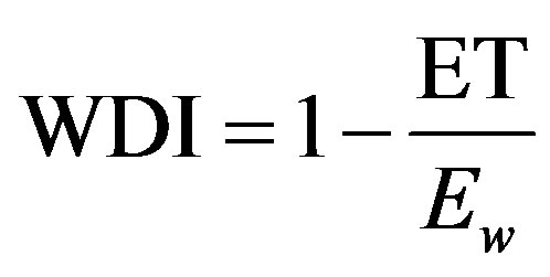
Moran et al. [8] provided the theoretical derivation of the WDI based on the relative evaporation, defined as the ratio between actual evapotranspiration (ET) and potential evapotranspiration (Epot). One of the main assumptions of the WDI is that soil and vegetation exchange energy and they cannot be analyzed separately [8]. This concept is particularly interesting for remote sensing applications where mix pixels, i.e. soil + vegetation, provide a single signal in every electromagnetic wavelength. The calculation is based on the vegetation index (VI) and Ts space, introduced by Price [9]. The most common VI used is the Normalized Difference Vegetation Index (NDVI) [10-12]. The IV-Ts space has also been used to estimate ET [13-15].
In this work we propose a new form of the WDI based on Jiang and Islam [16], and Priestley and Taylor [17] methods. The theoretical background provided by Moran et al. [8] is consistent to Jiang and Islam [16] methodology to estimate ET, therefore they are linkable in a single index called WSIEw.
2. Methodology
The background methodologies are the WDI published by Moran et al. [8] and Jiang and Islam [16] method. In this session both methods are briefly presented before we present the rationale behind the new index.
2.1. The WDI Index
Moran et al. [8] discussed the validity of the CWSI theory for partially vegetated areas. The derivation of their new index is based on the interpretation of the trapezoidal shaped IV-(Ts-Ta) plot, where Ta is the air temperature.
Figure 1 exemplifies the borders of the trapezoid. The segment 1 - 3 represents the cold edge, with well watered conditions and vegetation cover ranging from bare soil to fully vegetated areas (NDVI ranging from 0 - 1). The segment 2 - 4, the warm edge, represents dry surfaces with vegetation varying from bare soil to full canopies. The segment 1 - 2 represents fully vegetated areas. Point 1 corresponds to well watered vegetation. Point 2 characterizes dry vegetation. The segment 3 - 4 represents bare soil [18]. Given the value of Ts-Ta at any point in the trapezoid (i.e. point B in Figure 1), the evaporation can be obtained by from the distances AB and BC.
The WDI considers two important assumptions associated to the relationship between IV and the difference Ts-Ta. First, the authors assume that the difference Ts-Ta is linearly related to percentage of vegetated area and the canopy and soil temperatures. Another important statement made by the authors is that given a certain net energy (Rn), the temperature of the foliage and soil are linearly related to the transpiration and evaporation respectively. Therefore, the variations in Ts-Ta would be associated to ET. Thus, for a partially vegetated area,
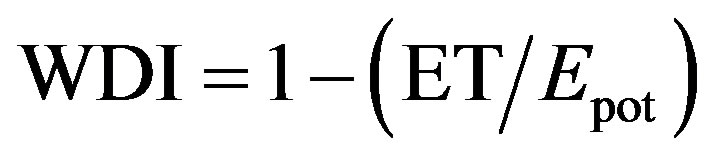 (1)
(1)
where (ET/Epot) is the relative evaporation. Epot is associated to a surface with unlimited water supply. The authors computed it with Penman-Monteith´s equation [19] assuming the vegetation resistance (rcp) closes to zero, without being canceled out.
Moran et al. [8] asserted that the VI has to be sensitive to the canopy variations and insensitive to spectral changes in soil background. Hence, the soil-adjusted vegetation index (SAVI) was the selected VI, and the linear
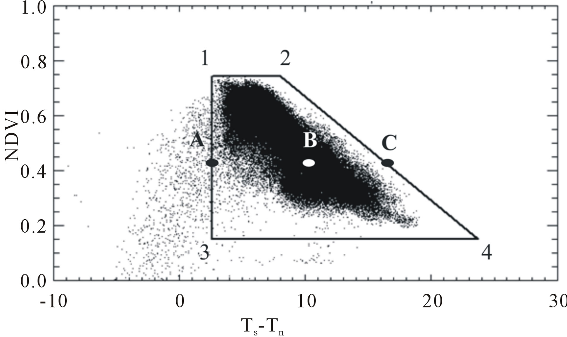
Figure 1. Trapezoidal diagram NDVI-(Ts-Ta) for date 04/05/ 2011.
edges of the SAVI-Ts space were adjusted to determine ET/Epot. Details of the WDI are provided in Moran et al. [8].
2.2. Jiang and Islam Method
The Jiang-Islam’s interpretation of the NDVI-Ts relationship provides the basis to estimate ET by modifying Priestley and Taylor’s equation [17]. Jiang and Islam introduced a coefficient to account for unsaturated areas, which replaced the original Priestley and Taylor’s coefficient (α). The resulting modified equation is,
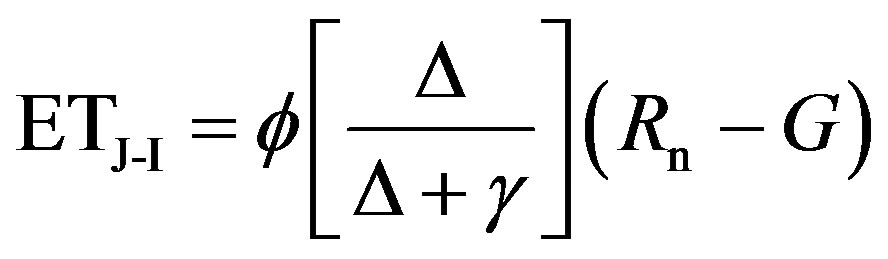 (2)
(2)
where f is Jiang-Islam’s parameter, Δ is the slope of the saturation vapor pressure curve, γ is the psychrometric constant, Rn is the net radiation at the surface level = and G is soil heat flux.
The parameter f varies from zero, for a dry bare soil surface, to α for a saturated or well vegetated surface, i.e. it becomes equal to Priestley and Taylor’s equation. This parameter f is calculated by a simple two-step linear interpolation between the sides of the NDVI-Ts triangle, as shown in Figure 2.
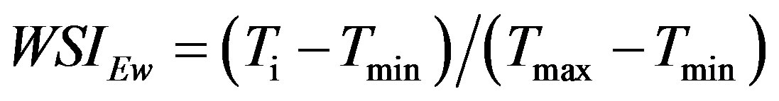
Jiang and Islam interpreted the upper edge, with high temperatures and low values of f, as the minimum value of ET for each class of NDVI, while the cold edge, associated with low Ts and maximum values of f, represents maximum ET rate. Therefore, the value of f vary within the limits of the triangle. Thus, NDVI-Ts plot is applied to derive f by using the normalized temperature,
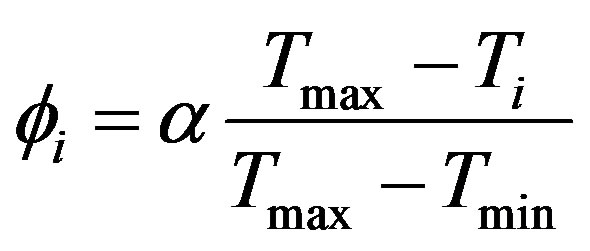 (3)
(3)
where Tmax and Tmin are the maximum and minimum Ts for a given vegetation class and Ti is the radiometric temperature for a given pixel.
In practice, the value of Tmax is the temperature obtained extrapolating the upper edge to intersect the Ts
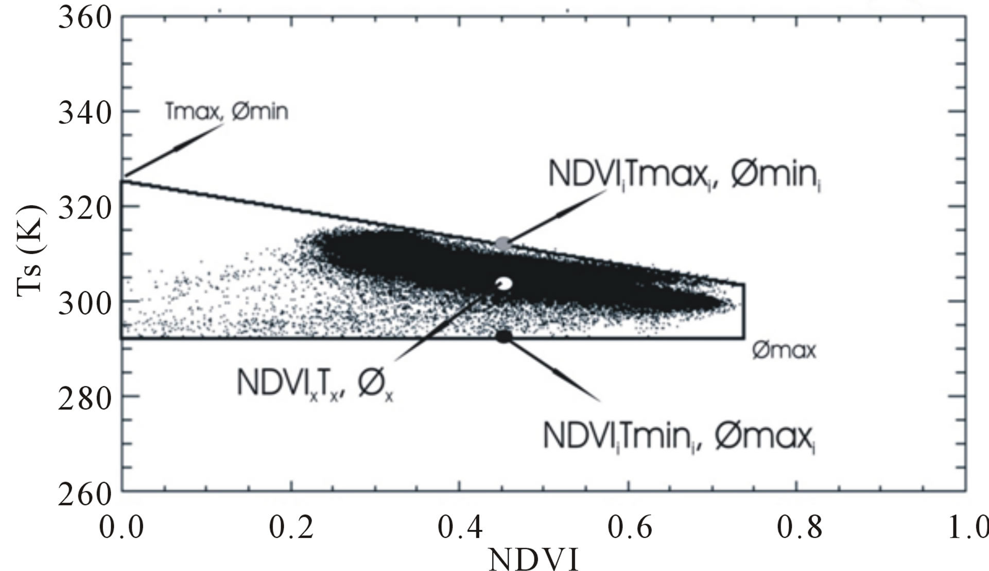
Figure 2. NDVI-Ts triangle space with upper and lower bonds and Jiang-Islam’s parameters for date 04/05/2011.
axis (Figure 2) for a NDVI = 0, while Tmin is obtained as the average Ts of those pixels identified as water, i.e. with NDVI < 0. A full description of f calculation can be found in Jiang and Islam [16].
2.3. The New Water Status Index (WSIEw)
Moran et al. [8] related the WS with ET/Epot (see equation (1)), where Epot was defined from the PenmanMonteith’s equation [19] suggesting that the Rn, Ta, vapor pressure deficit (VPD) and the soil moisture (SM) are the main controlling factors for the stomata opening [2,4,8]. One of the main assumption of this model is that rcp tends to zero. This Epot definition is closer to a wet environment evapotranspiration (Ew) concept than to a truly potential concept, where the energy is maximum, the surrounding air is dry while the surface is saturated [20]. Hence, for a given atmospheric condition and unlimited water supply, the soil+ plant complex will evapotranspire at its maximum rate according to the available energy. In this case, the maximum rate of ET is given by Ew [17,21-23].
The vegetation stress is mainly caused by deficit of moisture at the root zone. In the absence of watering, the moisture content in the root zone will be reduced as a result of crop intake. In turn, water stress causes the closure of the stoma of the plants and hence a reduction in the transpiration rate. Then, the ratio ET/Ew is a good indicator of evapotranspiration deficit [24]. Thus, Ew can replace the Epot in equation (1), and the WDI (see equation (1)) can be written as,
 (4)
(4)
In this new form of WDI, ET can be replaced by the equation (2) [16] and Ew by the Priestley-Taylor equation. The new index, WSIEw in terms of the parameters f and a is:
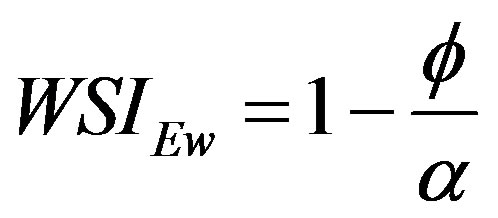 (5)
(5)
replacing f by equation 3,Traducir del: españolEscribe texto o la dirección de un sitio web, o bien, traduce un documento.CancelAlpha the WSIEw becomes,
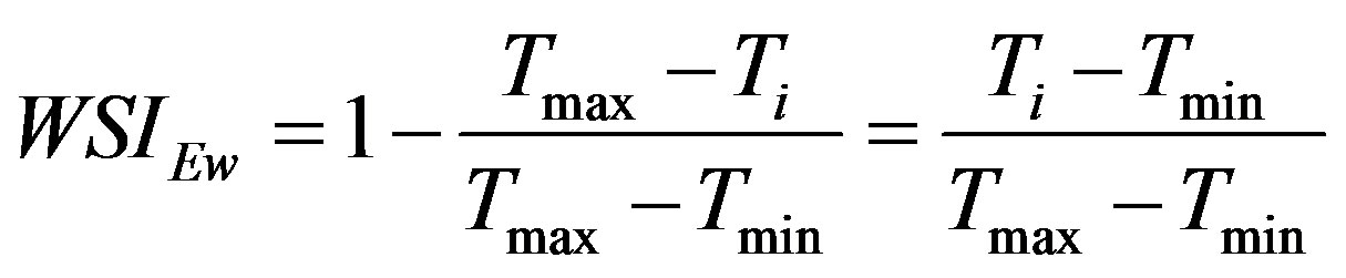 (6)
(6)
where Ti is the radiometric temperature for a given pixel and Tmax and Tmin are the Jiang and Islam’s parameters.
Operational robust methods could be achieved with purely remotely sensed data, as we propose here. In this case, Ta and the VPD are not explicitly required to compute the new index. The WSIEw does not require the understanding of the crop type biophysical functions under specific climates. The WSIEw could be calculated from data recorded from current satellite missions, such as NOAA series, EOS-Terra and EOS-Aqua. In this work we applied to WSIEw to the Southern Great Plains (SPG), using MODIS images and comparing the results with observations.
3. Study Area and Data
3.1. Study Area
The SGP region of US is a flat terrain, heterogeneous land cover with seasonal variation in temperature and humidity. It extends over the State of Oklahoma and southern part of Kansas, running from longitude 95.5˚W to 99.5˚W and from latitude 34.5˚N to 38.5˚N.
This region has relatively extensive and well distributed coverage of ground stations, maintained by the Atmospheric Radiation Measurement (ARM) program. The stations are widely distributed over the whole domain (Figure 3). E8 and E22 are located in a grazed rangeland region, E4 in an ungrazed rangeland area, E13 is positioned in a region with pasture and wheat, E7, E9, E15, E20 and E27 are located in pastures. E18 and E19 are in ungrazed pasture area, E12 is located in a native prairie, E10 is in alfalfa, E16 is in wheat region and E2 is in grass region.
3.2. Data and Images
The Energy Balance Bowen Ratio (EBBR) system compute 30-min estimates of the sensible and latent heat vertical fluxes at the local scale. Flux estimates are calculated from observations of net radiation, soil surface heat flux, and the vertical gradients of temperature and relative humidity. The instruments and measurement applications are well established and have been used for validation purposes in many studies [22,23,25,26]. Further information about the ARM EBBR data and methodology is available at http://www.arm.gov.
MODIS is one of the instruments on board EOS-Terra and EOS-Aqua satellites http://modis.gsfc.nasa.gov/ [27,28].
Daytime MODIS-Aqua images for nine days in years 2009, 2010 and 2011 in spring and summer with at least 82% of the study area free of clouds were selected. Table 1 summarizes the image information including date, day of the year, satellite overpass time and image quality. The product MYD02 and MYD11 were used in this work. MYD02 provides corrected radiance, reflectance and geolocations for 36 bands and MYD11 provides Ts images on a daily base [23,29,30].
4. Results
4.1. Preprocessing
The MODIS images were georeferenced from the Latitude and Longitude associate to each pixel. The study area was pulled out of each image and geographically projected in a grid of 445 columns by 445 rows, with
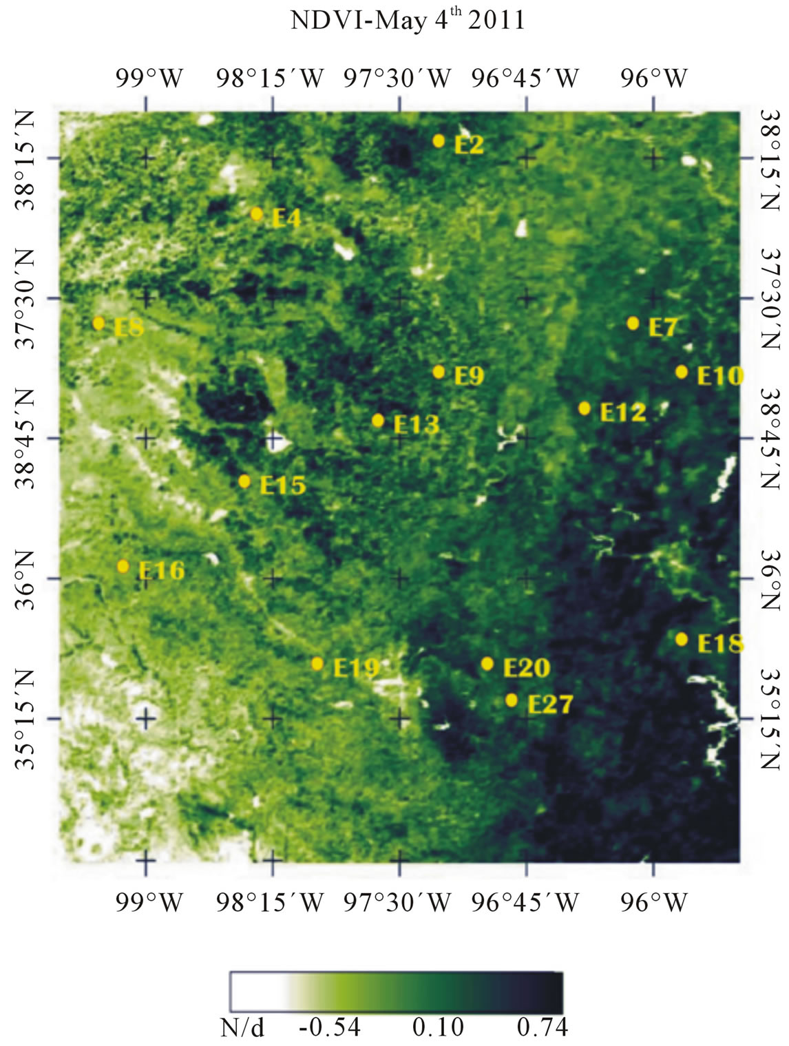
Figure 3. Southern Great Plains and ground station locations.
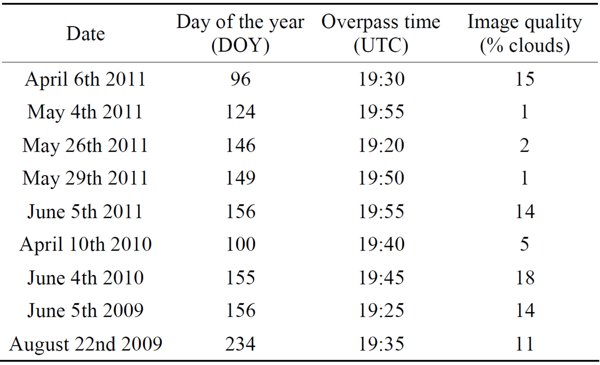
Table 1. Date day of the year overpass time and image quality of the nine study days.
pixels of approximately 1 km resolution. The reflectance of the red band (R) and near-infrared band (NIR) were obtained at the top of the atmosphere. The R and NIR images were used to obtain the NDVI,
 (7)
(7)
The NDVI-Ts spaces were plotted to obtain Jiang-Islam’s parameters (Tmax and Tmin) and then obtain the WSIEw by equation (6). Then, the WSIEw was validated with field data and contrasted with variables that are commonly associated to water stress.
Given that the WS is not directly measurable, we computed the WS with equation (4) using ET ground observations (ETobs) and Pristley and Taylor’s equation as follows,
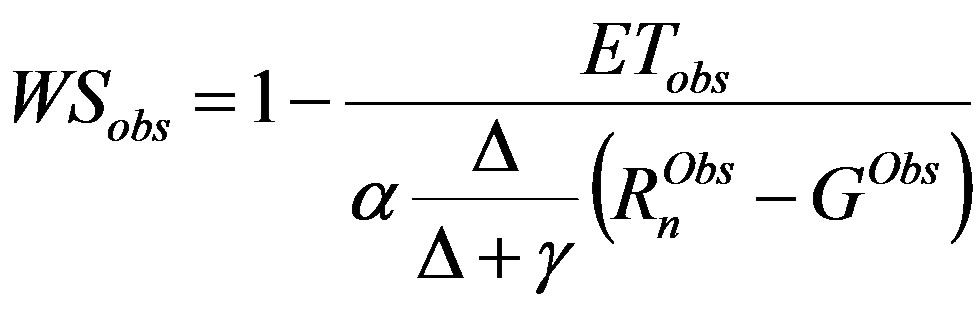 (8)
(8)
where  is the net radiation observed at the bowen ratio stations,
  is the ground data of soil head flux, D and g were computed from observed air temperature and atmospheric pressure.
WSIEw was compared with the WSobs and WDI obtained from NDVI-(Ts-Ta) space. Finally, in order to analyze the applicability of WSIEw we compared it with different variables associated to the stress.
4.2. WS Results
The regional statistic of WSIEw, i.e. maximum, mean and standard deviation, for each of the days are shown in Table 2.
The regional minimum is always equal to 0.0, since Jiang and Islam’s method [16] requires free water pixels to estimate Tmin. The minimum temperature represents ET = Ew, i.e. no-stress condition; thus, no-stress pixels are always present in this methodology. The regional maximum ranges from 0.50 and 0.72. The mean values of WSIEw vary from 0.14 to 0.42. For all the study days, the standard deviation is lower than 0.12 suggesting little regional dispersion around the mean of WSIEw. Wang et al. [12] analyzed the phenological cycle of winter wheat under irrigation in the North China Plain. The authors associated CWSI values lower than 0.34 to no stress conditions. Kar and Kumar [31] analyzed the CWSI in peanut crops under irrigation. They found CWSI values between 0.61 and 0.63 just before the application of irrigation. Hence, the regional WSIEw obtained here are comparables with those published by other authors. How-ever further analysis is needed to characterize the
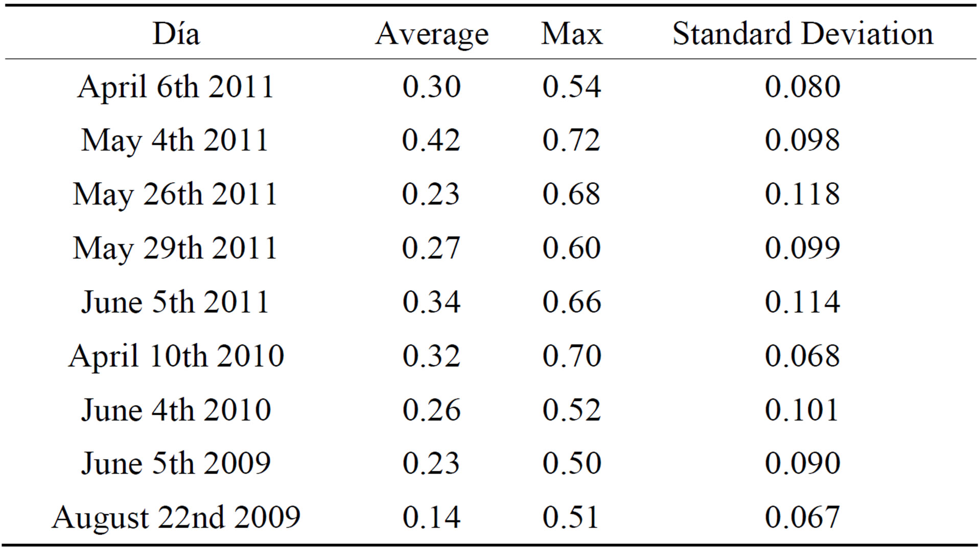
Table 2. regional statistics WSIEw (values maximum, average and standard deviation).
WSIEw valid range.
Results of WSIEw and WSobs were compared. The bias was obtained as ∑(WSobs − WSIEw)/n and RMSE as (∑(WSobs − WSIEw)2/n)0.5, where n is the number of observations. These statistics show bias of 0.05 and RMSE of 0.120, which represents approximately 24% of the mean WS (assuming a mean value of 0.5).
It is not evident how to validate the stress indexes from the literature revised here. For instance, Colaizzi et al. [32] compared the WDI and the soil water deficit index (SWDI). They found values of RMSE lower than 0,143 (29% of the mean) and bias lower than 0.112, consistent with the results presented here. In both cases, the RMSE are of the same order indicating that the method’s errors are about 30% of the mean.
The comparison between WDI and WSIEw remarks the differences between both models, with a bias of 0.28 and RMSE of 0.27 (54%). These results could be due to the separation between the bulk of the pixels and the dry border in the trapezoid (see Figure 1). These differences would be related to the differences in the Ew and Epot concepts already explained in Section 2.3.
The WSIEw results were also compared with records of different variables that index water stress. Figure 4 presents the WSIEw versus observed SM (at 5 cm below the surface).
There is a well defined inverse relationship between the SM and the WSIEw (Figure 4) with a coefficient of determination (R2) equal to 0.52. The dissimilar spatial resolution of both data sets may be the cause of the dispersion observed in Figure 4. Certainly the WSIEw is calculated as a result of the signal from 1 km × 1 km pixel while the ancillary data are representative of few meters around the point station [30]. Nevertheless, values of SM of 5%, characteristic of low moisture in most soils, correspond to WSIEw of about 0.45 while a SM of 30%, i.e. a well watered surface, could be associated to a WSIEw of 0.2.
Figure 5 displays WSIEw versus Tsoil (at 5 cm below the surface). These relationship showed a R2 = 0.72. It should be noted that f is a dimensionless temperature, what may explain the relationship with the soil temperature presented in Figure 5. Patel et al. [33] examined the potential of using canopy-air temperature difference (Tc-Ta) for assessing the crop water status. The authors correlated Tc-Ta with SM (at 15 cm) with a R2 = 0.59. Fensholt and Sandholt [34] found a R2 = 0.48 when comparing the Shortwave Infrared Water Stress Index (SIWSI) with soil moisture observed in situ.
The inverse relationship between observed ETobs and calculated WSIEw presented in Figure 6 is noteworthy, given that the ET records are independent to ETJ-I/Ew. In general, the WSIEw seems to capture the surface water stress condition well.
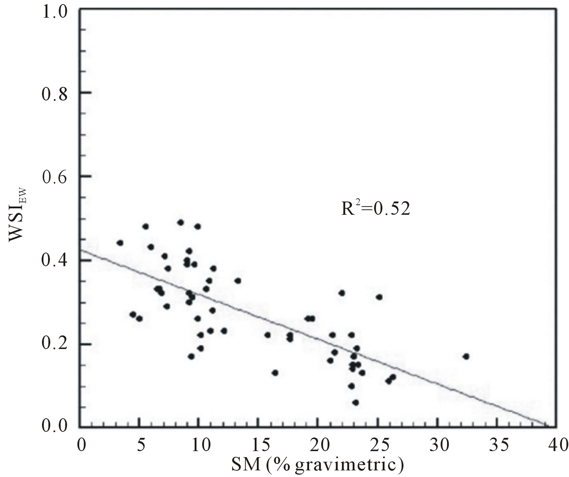
Figure 4. WSIEw vs observed SM (at 5 cm).
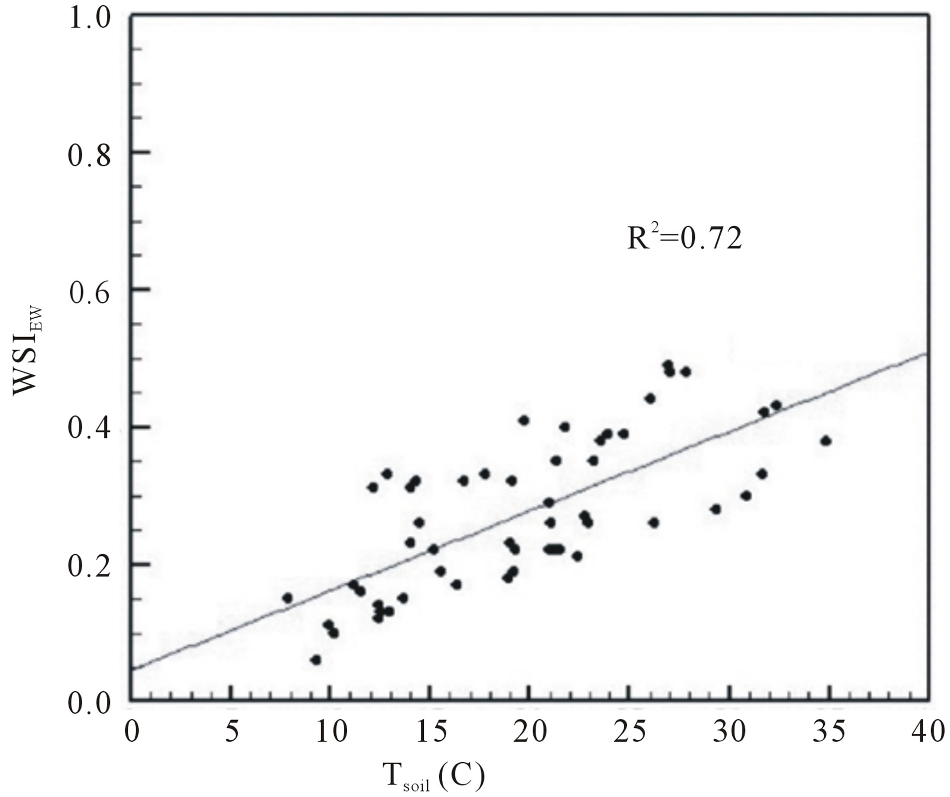
Figure 5. WSIEw vs observed Tsoil (at 5 cm).
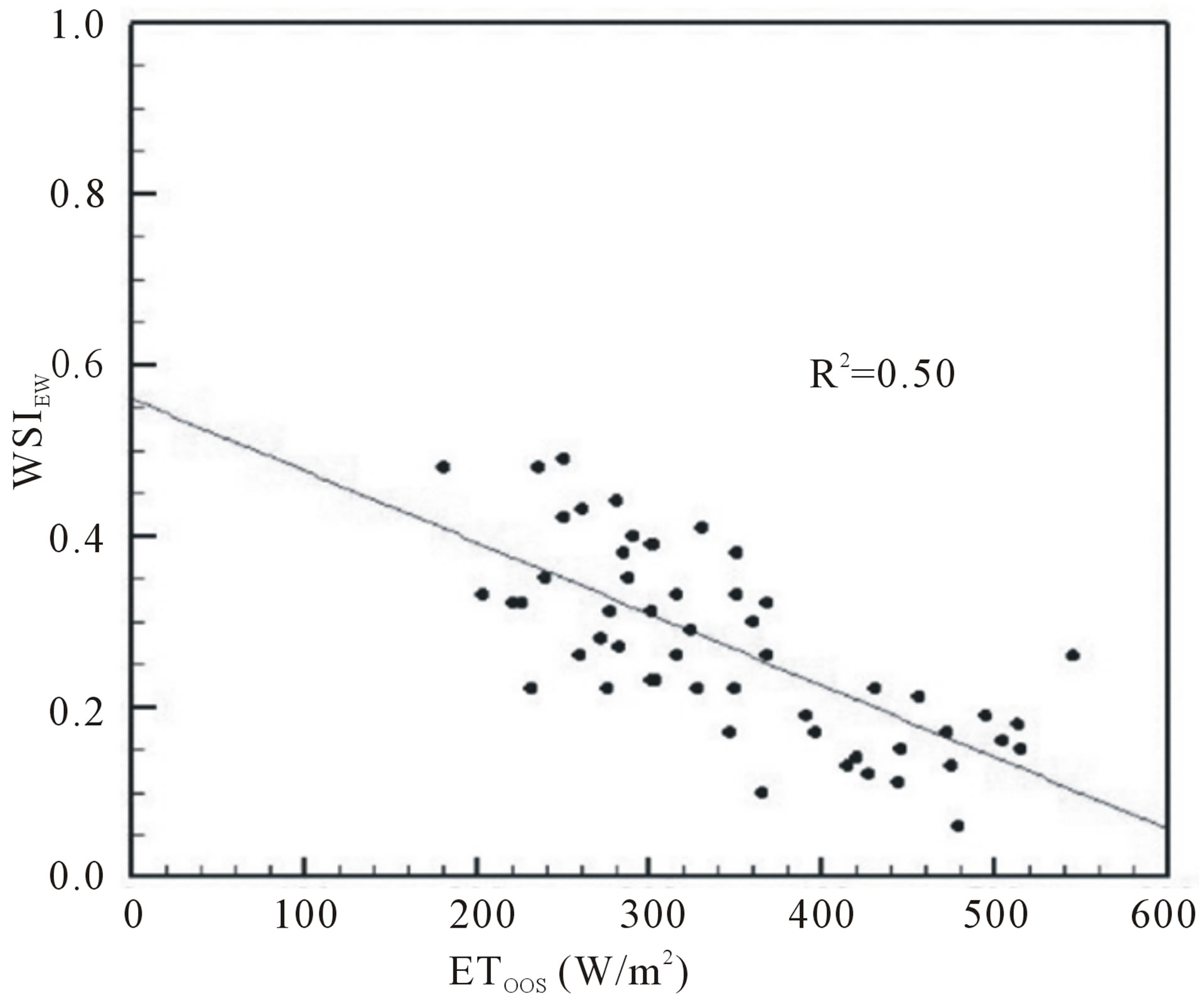
Figure 6. WSIEw vs observed ET.
The WSIEw was compared with the rainfall accumulated five days prior to the analyzed dates (PP). The comparison is shown in Figure 7 where the decrease of WS when rainfall increases is observed (R2 = 0.62). As the surface gets humid more water is available for ET and the ratio ET/Epot tends to one. Thus, the stress decreases with the precipitation increase.
Wang et al. [12] studied the wheat in the plain of China. They associated the wheat low stress to high rainfall events. The authors concluded that a good wheat harvest was obtained for CWSI lower than 0.34, representing a not-stress condition.
Figure 8 shows the comparison of WSIEw with soil moisture and PP for station E12. The SM observed at 5 cm is supplied by PP and represent the roots water availability [34], thus any reduction of PP, causes a decrease in the SM and it is expected to cause an increase of the WSIEw.
Finally, Figure 9 shows the WSIEw map for the SGP for the May 4th 2011, where we observed the stress would decreases from West to East. In general, the mountain areas present WSIEw of 0.7 and the prairies at the East show values of WSIEw about 0.3. The black areas are cloudy masked pixel [16,30].
4.3. Sensitivity Analysis
Tmax is the main parameter of the index presented in this paper, thus the sensitivity of the WSIEw to variation of Tmax is analyzed here.
Different methods to draw the warm and cold edge of the triangle [10,11] would render different values of Tmax in Jiang-Islam method. Thus, we apply the First Order Analysis to estimate the effect of Tmax on WSIEw variance.
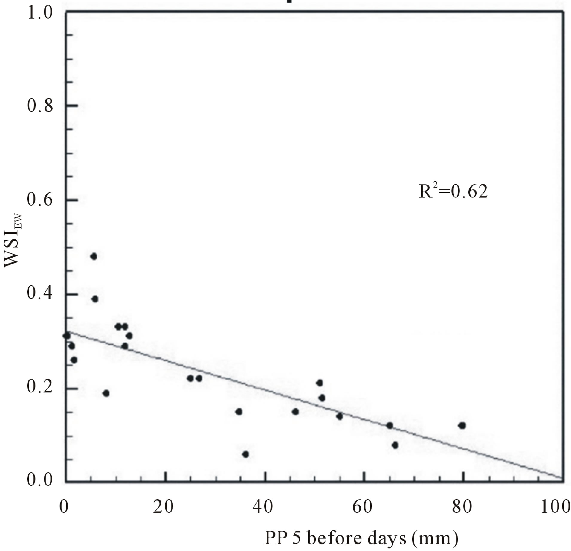
Figure 7. WSIEw vs PP (mm).
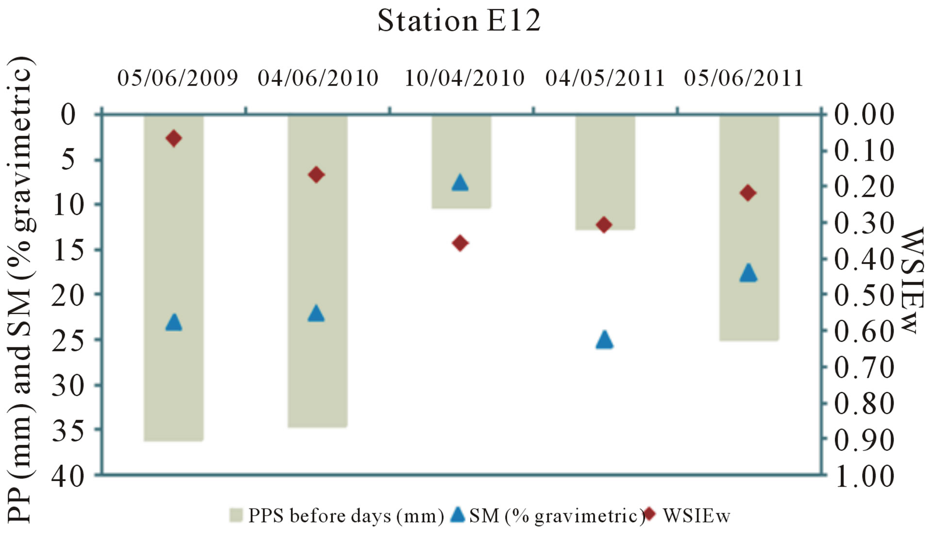
Figure 8. WSIEw vs SM and PP for station E12.
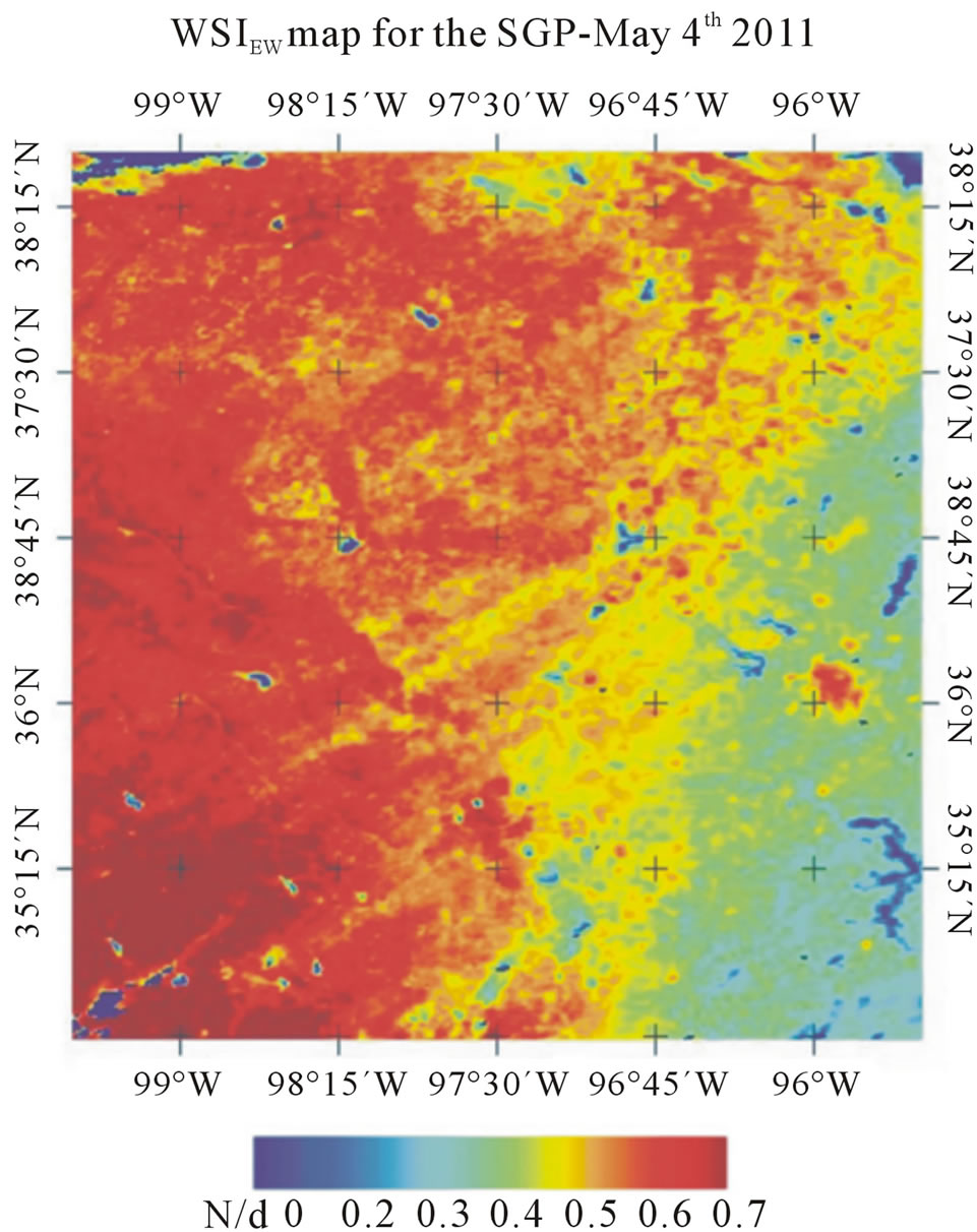
Figure 9. WSIEw map for the SGP for the May 4th 2011.
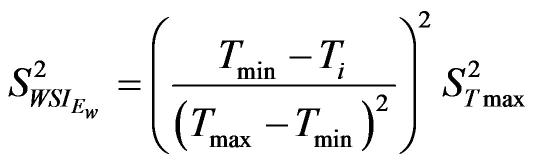 (9)
(9)
The results of applying equation (9) with differents Tmin, Tmax, Ti statistic and assuming that  varies from 1% to 15%, suggested that
  varies from 2.5% to 30% approximately. These results indicate that variations up 10% of Tmax would cause errors of about 15% in WSIEw.
5. Discussion
Several methods have been developed to determine the WS from observations of the Ts [2-5]. The index proposed by Moran et al. [8], based on the relative evaporation concept, is widely applied all over the world [18,32, 35]. In this work we presented a modification of WDI proposed by Moran et al. [8]. The new index replaces the Epot used in the original formulation for the Ew concept. Given that Ew £ Epot [20], the ratio ET/Epot is smaller than ET/Ew, yielding two WS indexes that point out different causes of vegetation stress. The WSIEw would only consider the stress due to water shortness in the root zone while the WDI would also reflect the stoma closure cause by the atmospheric and radiation effects.
The WDI required field information (observations of Rn, G, wind speed, Ta) to establish the end-points that define the trapezoid (Figure 1(a)). If such information was not available, it would be necessary to guess them from each analyzed image; i.e. indentifying groups of pixels that represent the natural conditions of the endpoints. Guessing the extreme points creates uncertainty in the interpretations of the diagrams [35]. The WSIEw also requires determination of the triangle borders, however in this case, the source of error would be mainly associated with definition of Tmax.
The WSIEw is another “thermal index” with the form of a normalized temperature, i.e.
[30]. Tmax is the temperature for a hypothetical dry bare soil pixel and Tmin is the temperature for a saturated pixel. It must be noted that the Tmax is not the maximum thermal infrared of the image or maximum canopy temperature; on contrast, it is a “hypothetical” maximum temperature. It is usually found in the literature thermal stress indices calculated as a normalized Ts, the difference between the methods is given the extreme temperatures estimation. For instance, Galleguillos et al. [18] used the WDI to derive the daily ET. The authors assumed that Ta is constant in the study area and they estimated the maximum and minimum Ts from the energy balance. Wang et al. [35] made used of the WDI to estimate soil moisture. These authors explored the Ts-EVI (Enhanced Vegetation Index) space to determine the minimum and maximum values of Ts.
The relationship between the WSIEw and SM (R2 = 0.52) provided interesting information. In Figure 3(a) we observe that a soil with 5% of moisture matches a WSIEw of about 0.45. On the other extreme, a SM of 30% agrees with a WSIEw of 0.1. In other words, the WSIEw would not get close to 1 although the SM indicates a dry surface.
We compare the WSIEw with the rainfall accumulated five days prior to the analyzed dates, observing that the WS decreases as precipitation increases, however there is no sufficient analysis about irrigation fields and precipitation spatial distribution in this work to deepen the conclusions about the WSIEw range of variation.
The advantage of this new formulation is that there is no need of crop-field observations, yet overestimated Tmax values might yield an underestimated water stress condition. Thus, a Tmax significantly larger than the actual dry soil temperature, would not index the stress with a WSIEw value close to 1, as it would be expected by the end-users. In general, the WSIEw shows significant correlations with water stress indicators.
The WSIEw is applicable to different satellite missions and requires minor image processing. The new index can be very useful for end users who require quick and easy methods of application.
REFERENCES
- R. López-López, R. Arteaga-Ramírez, M. A. VázquezPeña, I. López-Cruz and I. Sánchez-Cohen, “Índice de Estrés Hídrico Como un Indicador del Momento de Riego en Cultivos Agrícolas,” Agricultura Técnica en México, Vol. 35, No. 1, 2009, pp. 92-106.
- R. D. Jackson, S. B. Idso, R. J. Reginato and W. L. Ehrler, “Crop Temperature Reveals Stress,” Crop Soils, Vol. 29, No. 8, 1977, pp. 10-13.
- R. D. Jackson, “Canopy Temperature and Crop Water Stress,” In D. Hillel, Eds., Advances in Irrigation, Academic Press, New York, 1982, pp. 43-85.
- S. B. Idso, “Non-Water-Stressed Baselines: A Key to Measuring and Interpreting Plant Water Stress,” Agricultural Meteorology, Vol. 27, No. 1-2, 1982, pp. 59-70. http://dx.doi.org/10.1016/0002-1571(82)90020-6
- K. L. Clawson and B. L. Blad, “Infrared Thermometry for Scheduling Irrigation of Corn,” Agronomy Journal, Vol. 74, No. 3, 1982, pp. 311-316.
- M. Usman, A. Ahmad, S. Ahmad, M. Arshad, T. Khaliq, A. Wajid, K. Hussain, W. Nasim, T. Mehmood Chattha, R. Trethowan and G. Hoogenboom, “Development and Application of Crop Water Stress Index for Scheduling Irrigation in Cotton (Gossypium hirsutum L.) under Semiarid Environment,” Journal of Food Agriculture and Environment, Vol. 7, No. 3-4, 2009, pp. 386-391.
- B. L. Blad, D. G. Gardner, N. J. Watts and N. J. Rosenberg, “Remote Sensing of Crop Moisture Status,” Remote Sensing, Quart. 3, 1981, pp. 4-20.
- M. S. Moran, T. R. Clarke, Y. Inoue and A. Vidal, “Estimating Crop Water Deficit Using the Relation between Surface-Air Temperature and Spectral Vegetation Index,” Remote Sensing Environment, Vol. 49, No. 3, 1994, pp. 246-263. http://dx.doi.org/10.1016/0034-4257(94)90020-5
- J. C. Price, “Using Spatial Context in Satellite Data to Infer Regional Scale Evapotranspiration,” IEEE Transactions on Geoscience and Remote Sensing, Vol. 28, No. 5, 1990, pp. 940-948. http://dx.doi.org/10.1109/36.58983
- T. N. Carlson, R. R. Gillies and T. J. Schmugge, “An Interpretation of Methodologies for Indirect Measurement of Soil Water Content,” Agricultural and Forest Meteorology, Vol. 77, No. 3-4, 1995, pp. 191-205. http://dx.doi.org/10.1016/0168-1923(95)02261-U
- I. Sandholt, K. Rasmussen and J. Andersen, “A Simple Interpretation of the Surface Temperature/Vegetation Index Space for Assessment of Surface Moisture Status,” Remote Sensing Environment, Vol. 49, No. 3, 2002, pp. 246-263.
- L. Wang, G. Y. Qiu, X. Zhang and S. Chen, “Application of a New Method to Evaluate Crop Water Stress Index,” Irrigation Science, Vol. 24, No. 1, 2005, pp. 49-54. http://dx.doi.org/10.1007/s00271-005-0007-7
- R. R. Gillies, T. N. Carlson, J. Cui, W. P. Kustas and K. S. Humes, “A Verification of the ‘Triangle’ Method for Obtaining Surface Fluxes from Remote Measurements of the Normalized Difference Vegetation Index (NDVI) and Surface Radiant Temperature,” International Journal of Remote Sensing, Vol. 18, No. 15, 1997, pp. 3145-3166. http://dx.doi.org/10.1080/014311697217026
- L. Jiang and S. Islam, “A Methodology for Estimation of Surface Evapotranspiration over Large Areas Using Remote Sensing Observations,” Geophysical Research Letters, Vol. 26, No. 17, 1999, pp. 2773-2776. http://dx.doi.org/10.1029/1999GL006049
- S. Stisen, I. Sandholt, A. Norgaard, R. Fensholt and K. H. Jensen, “Combining the Triangle Method with Thermal Inertia to Estimate Regional Evapotranspiration—Applied to MSG-SEVIRI Data in the Senegal River Basin,” Remote Sensing Environment, Vol. 112, No. 3, 2008, pp. 1242-1255. http://dx.doi.org/10.1016/j.rse.2007.08.013
- L. Jiang and S. Islam, “Estimation of Surface Evaporation Map over Southern Great Plains Using Remote Sensing Data,” Water Resources Research, Vol. 37, No. 2, 2001, pp. 329-340. http://dx.doi.org/10.1029/2000WR900255
- C. H. B. Priestley and R. J. Taylor, “On the Assessment of Surface Heat Flux and Evaporation Using Large-Scale Parameters,” Monthly Weather Review, Vol. 100, No. 2, 1972, pp. 81-92. http://dx.doi.org/10.1175/1520-0493(1972)100<0081:OTAOSH>2.3.CO;2
- M. Galleguillos, F. Jacob, L. Prévot, A. French and P. Lagacherie, “Comparison of Two Temperature Differencing Methods to Estimate Daily Evapotranspiration over a Mediterranean Vineyard Watershed from ASTER Data,” Remote Sensing Environment, Vol. 115, No. 6, 2011, pp. 1326-1340. http://dx.doi.org/10.1016/j.rse.2011.01.013
- J. L. Monteith and M. Unsworth, “Principles of Environmental Physics,” 2nd Edition, Butterworth-Heinemann, Burlington, 1990, 304p.
- R. J. Granger, “An Examination of the Concept of Potential Evaporation,” Journal of Hydrology, Vol. 111, No. 1-4, 1989, pp. 9-19. http://dx.doi.org/10.1016/0022-1694(89)90248-5
- W. Brutsaert and H. Stricker, “An Advection-Aridity Approach to Estimate Actual Regional Evapotranspiration,” Water Resources Research, Vol. 15, No. 2, 1979, pp. 443-450. http://dx.doi.org/10.1029/WR015i002p00443
- V. Venturini, S. Islam and L. Rodríguez, “Estimation of Evaporative Fraction and Evapotranspiration from MODIS Products Using a Complementary Based Model,” Remote Sensing Environment, Vol. 112, No. 1, 2008, pp. 132-141. http://dx.doi.org/10.1016/j.rse.2007.04.014
- V. Venturini, L. Rodríguez and G. Bisht, “A Comparison among Different Modified Priestley and Taylor’s Equations to Calculate Actual Evapotranspiration with MODIS Data,” International Journal of Remote Sensing, Vol. 32, No. 5, 2010, pp. 1319-1338. http://dx.doi.org/10.1080/01431160903547965
- J. V. Straschnoy, C. M. Di Bella, F. R. Jaimes, P. A. Oricchio and C. M. Rebella, “Caracterización Espacial del Estrés Hídrico y de las Heladas en la Región Pampeana a Partir de Información Satelital y Complementaria,” Revista de Investigaciones Agropecuarias, Vol. 35, No. 2, 2006, pp. 117-141.
- W. J. Shuttleworth, “Insight from Large-Scale Observational Studies of Land/Atmosphere Interactions,” Surveys in Geophysics, Vol. 12, No. 1-3, 1991, pp. 3-30. http://dx.doi.org/10.1007/BF01903410
- J. M. Lewis, “The Story behind the Bowen Ratio,” Bulletin of the American Meteorological Society, Vol. 76, No. 12, 1995, pp. 2433-2443. http://dx.doi.org/10.1175/1520-0477(1995)076<2433:TSBTBR>2.0.CO;2
- C. O. Justice, J. R. G. Townshend, E. F. Vermote, E. Masuoka, R. E. Wolfe, N. Saleous, D. P. Roy and J. T. Morisette, “An Overview of MODIS Land Data Processing and Product Status,” Remote Sensing Environment, Vol. 83, No. 2, 2002, pp. 3-15.
- E. F. Vermote, N. Z. Saleous and C. O. Justice, “Atmospheric Correction of MODIS Data in the Visible to Middle Infrared: First Results,” Remote Sensing Environment Vol. 83, No. 2, 2002, pp. 97-111.
- Z. Wan and J. A. Dozier, “A Generalized Split-Window Algorithm for Retrieving Land-Surface Temperature from Space,” IEEE Transactions on Geoscience and Remote Sensing, Vol. 34, No. 4, 1996, pp. 892-905. http://dx.doi.org/10.1109/36.508406
- V. Venturini, G. Bisht, S. Islam and L. Jiang, “Comparison of Evaporative Fractions Estimated from AVHRR and MODIS Sensors over South Florida,” Remote Sensing Environment, Vol. 93, No. 1-2, 2004, pp. 77-86. http://dx.doi.org/10.1016/j.rse.2004.06.020
- G. Kar and A. Kumar, “Surface Energy Fluxes and Crop Water Stress Index in Groundnut under Irrigated Ecosystem,” Agricultural and Forest Meteorology, Vol. 146, No. 1-2, 2007, pp. 94-106. http://dx.doi.org/10.1016/j.agrformet.2007.05.008
- P. D. Colaizzi, E. M. Barnes, T. R. Clarke, C. Y. Choi, M. Peter, P. M. Waller, J. Haberland and M. Kostrzews, “Water Stress Detection Under High Frequency Sprinkler Irrigation with Water Deficit Index,” Journal of Irrigation and Drainage Engineering, Vol. 129, No. 1, 2003, pp. 36- 43.
- N. R. Patel, A. N. Mehta and A. M. Shekh, “Canopy Temperature and Water Stress Quantificaiton in Rainfed Pigeonpea (Cajanus cajan (L.) Millsp.),” Agricultural and Forest Meteorology, Vol. 109, No. 3, 2001, pp. 223- 232. http://dx.doi.org/10.1016/S0168-1923(01)00260-X
- R. Fensholt and I. Sandholt, “Derivation of a Shortwave Infrared Water Stress Index from MODIS Nearand Shortwave Infrared Data in a Semiarid Environment,” Remote Sensing Environment, Vol. 87, No. 1, 2003, pp. 111-121. http://dx.doi.org/10.1016/j.rse.2003.07.002
- W. Wang, D. Huang, X. G. Wang, Y. R. Liu and F. Zhou, “Estimation of Soil Moisture Using Trapezoidal Relationship between Remotely Sensed Land Surface Temperature and Vegetation Index,” Hydrology and Earth System Sciences, Vol. 15, No. 5, 2011, pp. 1699-1712. http://dx.doi.org/10.5194/hess-15-1699-2011
NOTES
*Corresponding author.