Computational Water, Energy, and Environmental Engineering
Vol. 2 No. 2 (2013) , Article ID: 30593 , 12 pages DOI:10.4236/cweee.2013.22004
Fundamentals of Direct Inverse CFD Modeling to Detect Air Pollution Sources in Urban Areas
Department of Environmental Engineering, Egypt-Japan University of Science and Technology (E-JUST), New Borg El-Arab City, Alexandria, Egypt
Email: mahmoud.bady@ejust.edu.eg
Copyright © 2013 Mahmoud Bady. This is an open access article distributed under the Creative Commons Attribution License, which permits unrestricted use, distribution, and reproduction in any medium, provided the original work is properly cited.
Received June 6, 2012; revised February 18, 2013; accepted February 25, 2013
Keywords: Inverse Modeling; Outdoor Environments; Reverse Simulation; CFD
ABSTRACT
This paper presents the fundamentals of direct inverse modeling using CFD simulations to detect air pollution sources in urban areas. Generally, there are four techniques used for detecting pollution sources: the analytical technique, the optimization technique, the probabilistic technique, and the direct technique. The study discusses the potentialities and limits of each technique, where the direct inverse technique is focused. Two examples of applying the direct inverse technique in detecting pollution source are introduced. The difficulties of applying the direct inverse technique are investigated. The study reveals that the direct technique is a promising tool for detecting air pollution source in urban environments. However, more efforts are still needed to overcome the difficulties explained in the study.
1. Introduction
Nowadays, inverse modeling seems to be a promising topic in terms of environmental research. The importance of reverse modeling arises from the increased numbers of pollution sources due to continuing industrial expansion coupled with population growth, especially in large cities. In addition, terrorist attacks are becoming more frequent and deadlier, such as the sarin gas attacks on the Tokyo subway in 1995, which resulted in 12 deaths and over 6000 injured [1,2], and the terrorist attacks on New York City and Washington DC on September 11, 2001 and the following anthrax dispersion by mail. Moreover, in the US, fire accidents occur in structures at the rate of one every 61 s, and in particular residential fires occur every 79 s. Nationwide, there was a civilian fire-related death every 156 minutes and a civilian fire-related injury every 28 minutes [3]. All of these events have confirmed that the terroristic attacks are no longer hypothesis but a reality. From this perspective, the ability to predict pollution sources characteristics: location, strength, and release time has become a necessity in order to create a complete picture of the air quality conditions within the release domain and to ensure the public’s safety. Inverse modeling using Computational Fluid Dynamics (CFD) simulations is one efficient and promising tool in this regard.
Traditionally, CFD is used to explore the cause-effect relationship that is called forward-time modeling. Inverse modeling is to find the causal characteristics such as the pollutant source location and strength from the finite effectual information like the distributions of airflow and pollutant concentrations. Generally, in modeling process, there are three different types of problems [4]:
• The forward-time problem: given input and system parameters, find out output of the model.
• The reconstruction problem: given system parameters and output, find out which input has led to this output.
• The identification problem: given input and output, determine the system parameters that agree with the relationship between input and output.
Type 1 problem is an oriented cause-effect sequence. In this sense, type 2 and 3 problems are inverse problems because they are the problems of finding unknown causes of known consequences.
In order to determine the pollution source within a domain through the use of inverse modeling, some measurements such as concentration distributions are needed to infer the values of the inputs or parameters that characterize the system [5]. In reality, the concentration field is obtained from data measured by concentration sensors. The conventional CFD codes predict airflow based on given inputs (boundary conditions) and system parameters (building and system characteristics), which is a forward-time problem. Then, the reverse simulation is carried out through the solution of the reversed transport equation using the measured concentration field and the solved air flow field.
By carrying out inverse CFD simulations, one can detect air pollution source (or release) characteristics. Identification of pollution sources immediately after release is a matter of urgency in order to ensure the public’s safety. Since, inverse modeling is one of the efficient and promising tools in this regard; this paper sheds light on the existing inverse techniques and explores the feasibility of using these techniques for urban environment study. Generally, there are four techniques used for detecting pollution sources the analytical technique, the optimizition technique, the probabilistic technique, and the direct inverse technique. First, the present study discusses the potentialities and limits of each technique. Then, the direct inverse modeling technique, as a promising tool to detect air pollution sources, is focused.
2. Different Techniques of Inverse Modeling
In the present study, the existing inverse modeling techniques that have been employed to detect pollutant sources in urban areas are reviewed. Figure 1 shows classification of inverse CFD modeling techniques. Each technique has its own advantage and disadvantage. In the following sections, the four techniques will be discussed in details.
2.1. The Analytical Approach
The analytical approach requires analytical solution of the distributions of airflow and pollutant concentrations. The causal characteristics are then inversely solved. The analytical approach has been successfully applied to multi-dimensional heat conduction problems [6]. In groundwater transport, the analytical approach has been used to solve contaminant transport in one-dimensional flow [7] or in 2-D uniform flow [8]. The analytical approach has also been used to solve an inverse atmospheric transport problem in three-dimensional uniform
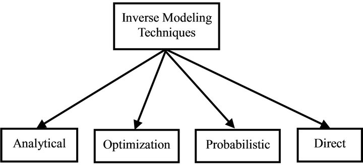
Figure 1. Classification of inverse CFD modeling techniques.
flow [9]. Using analytical and graphical techniques, Islam [10,11] worked out a method for determining an unknown emission source in urban areas based on the well known Gaussian Plume Model (GPM). He assumed that the GPM describes the dispersion process fully.
The above discussion shows that the analytical approach can be accurate and efficient. However, it is only used for simple problems. Accordingly, the application of the analytical approach in problems of complex geometry is very limited.
2.2. The Optimization Approach
In the optimization approach, forward-time modeling is used to obtain the effectual data (such as distributions of pollutant concentrations) based on all possible causal characteristics. Then the approach optimizes a solution that is best-fitted with the corresponding measured data. This approach has been widely applied in identifying groundwater pollution source as linear optimization method [12], maximum likelihood method [13], and nonlinear optimization method [14]. As an example, Arvelo et al. (2002) [6] have used a modified multi-zone model to study the optimal placement of chemical/biological warfare agent sensors in a building with nine offices and a hallway. The optimal sensor locations should be in the spaces where most possible sources of chemical/biological warfare agent could be located so the sensors can detect the agent in least amount of time. Different from the previous researchers, they used the genetic algorithm to interpret the computed data to locate the sources. Because plausible combinations of possible causal characteristics are huge, this approach involves a large amount of modeling.
2.3. The Probabilistic Approach
The probabilistic approach also does forward-time modeling. The approach uses probability to express a possible causal aspect. In groundwater transport, Bagtzoglou et al. (1992) [15] calculated the possibility of a contaminant source in groundwater by reversing only the convective contaminant transport. Other researchers [16] used Bayesian theory to interpret the possibility of each contaminant source. In enclosed environment, Sohn et al. (2002) [17] also used Bayesian probability model to identify the contaminant source in a five-room building. They used a multi-zonal model to calculate the airflow and contaminant transport. Since the multi-zone model can only provide some macroscopic information about the contaminant transport, it is necessary to run CFD simulations if more accurate and detailed information is needed. Accordingly, both the probability and optimization approaches need a huge amount of forward-time modeling.
2.4. The Direct Inverse Approach
The direct inverse approach solves inverse problems by reversing directly the governing equations that describe cause-effect relations. Kato et al. (1992) applied the reverse tracking of flow field over time, to obtain the residual lifetime of air at a point. In addition, Kato et al. [18-20] used the same technique to assess local pollution from upwind regions with backward trajectory analysis of the flows in an atmospheric environment. They reversed only the pollutant transport by convection and neglected the effect of diffusion. The method has also been used in groundwater contaminant transport [15,21], where convection transport of pollutants is solved with reversed velocity field and the diffusion was left unchanged.
In the following sections, the direct inverse modeling technique is investigated in details. The fundamentals of the technique are introduced. Then, the difficulties in applying the technique are discussed. Finally, two examples of applying the direct inverse technique in detecting pollution source in urban area are introduced.
3. Fundamentals of Direct Inverse Modeling
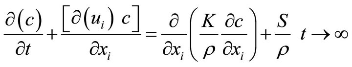
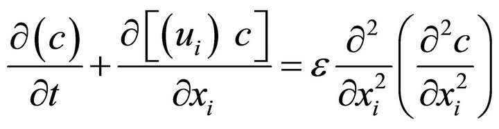
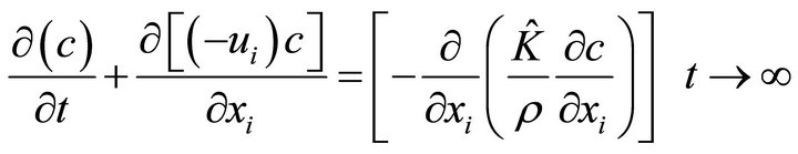
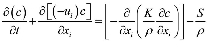
Pollutant concentrations are predicted based on the convection-diffusion equation including meteorological data, transport diffusion, and the relevant emissions (S). It can be written as follows [22]:
 (1)
(1)
where c is the pollutant concentration (kg/kg)t is the time (s)ui is the Cartesian components of the velocity (m/s)xi is the Cartesian coordinates (m)K is the concentration diffusivity coefficient (kg/m/s)ρ is the air density (kg/m3), and S is the pollutant source strength (kg/m3/s).
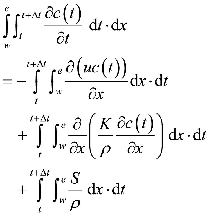
In order to explain the principles of inverse modeling, Equation (1) can be simply integrated based on one dimensional flow as shown in Figure 2 with using upwind scheme for space:
 (2)
(2)
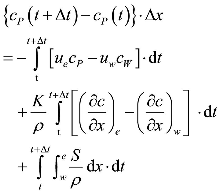
Assuming K and ρ to be constant, the integration result becomes:
 (3)
(3)
Rearranging Equation (3), then:
 (4)
(4)
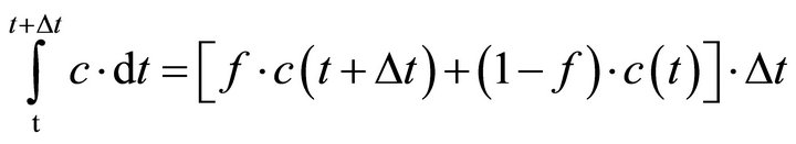
To perform the integration with respect to time, the concentration-time relation is needed. Usually, the following equation is assumed [23]:
 (5)
(5)
where f is a weighting factor used to combine the concentration value at the new time step with both of new and old concentration values.
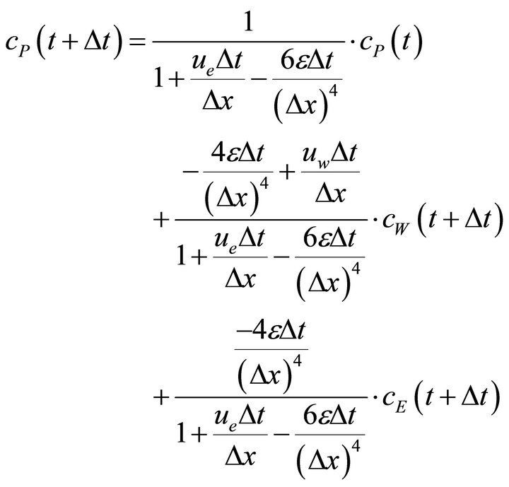
By applying fully implicit scheme (i.e. f = 1), Equation (5) can be rearranged to the form:
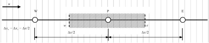
Figure 2. Typical control volume for the one-dimensional flow.
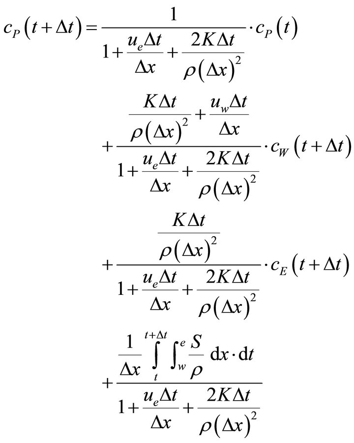 (6)
(6)
Clearly, in order to calculate the concentration at previous time, one can simply apply a negative time step in Equation (1). However, the negative time step makes the coefficient of cP(t) greater than one, which amplifies the calculation errors as time elapsed in negative direction. Thus, Equation (1) is unstable in inverse modeling. Accordingly, in order to solve the reverse transport equation with numerical stability, another approach has to be used. One of these approaches is to use a slightly different equation instead of the original equation [24-26].
The inverse direct technique requires less-efforts compared with the probabilistic technique and the optimization technique. However, the instability problem caused by the negative diffusion term represents the main difficulty when applying such technique. This will be investigated in the following section.
4. Solution Instability in Direct Approach
Since the reversed governing equations are unstable due to the negative diffusion term, many researchers have worked out to improve the solution stability through imposing a bound on the solution. The regularization technique (or the stabilization technique) has been used to improve the solution stability. The solution is obtained by minimizing the objective function with a regularized term. The stabilization technique introduces some stabilization terms into the reversed governing equations or solves some auxiliary equations to improve the solution stability. For example, Zhang and Chen (2007) [26] and Liu et al. (2011) [27] changed the diffusion term in the reversed transport equation as (i.e. Equation (1)):
 (7)
(7)
where ε is a stabilization coefficient.
The equation is numerically stable compared with Equation (6), since the coefficient of cP can be smaller than one, where:
 (8)
(8)
The required condition is just to make ε larger than ue∆x3/6, which is easy to be satisfied. Then the numerical scheme becomes stable and the reversed transport equation becomes dispersive.
By comparing the stabilization and the regularization methods, Skaggs and Kabala (1995) [25] concluded that the stabilization method used significantly less computational effort than the regularization method, although the stabilization method might provide slightly inferior results.
In the present study, in order to make the equation solvable with numerical stability, this study proposes the use of a filter to deal with negative concentration gradients in order to avoid unrealistic solutions. Then, Equation (1) can be rewritten as:
 (9)
(9)
where the symbol “ˆ” means that this term is filtered.
The filter for the diffusion term is set in such a way that the negative concentration values are changed to the minimum positive value of the concentration within the solution domain. This can be expressed as:
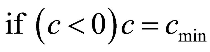 (10)
(10)
Indeed, the filtration process of the diffusion term in the reversed transport equation affects the solution accuracy and decreases the method’s effectiveness in identifying the sources of pollution. This will be investigated in the following examples.
5. Examples of Applying Direct Inverse Modeling in Identifying Source Locations
5.1. Simple Laminar Flow
A 3-D numerical model for modeling a simple laminar flow is designed as shown in Figure 3. The dimensions of the computational domain are 90 m × 30 m × 30 m (L × W × H). The minimal mesh size above the ground is set as 0.18 m, and the vertical growing factor for mesh points is 1.05. The total number of cells is 594,000. A pollution source of strength 0.01 kg/m3/s and dimensions 0.5 m × 0.5 m × 0.5 m is considered at a location 12 m from the inlet face at a height of 2 m.
5.2. Turbulent Flow around a Single Building
The second example for identifying the source of pollution in urban areas using direct inverse modeling is shown in Figure 4, in which wind flows around a single building. The building dimensions are 10(x) × 10(y) × 30(z) m and the computational domain dimensions are 300(x) × 110(y) × 70(z) m with a mesh size of 444,800 cells.
Two different locations for the source are considered in order to examine the effect of pollutant source location on the prediction accuracy of the reverse technique: location (I), which is 2.5 m upwind the building, and location (II), which is 2.5 m downwind the building. In both cases, the source strength is set at 0.01 kg/m3/s with dimensions of 0.5 m × 0.5 m × 0.6 m.
5.3. Numerical Simulation
Numerical simulations are carried out using the CFD code Star-CD, based on the finite-volume discretization method. During forward-time simulation, steady-state analysis is adopted for the flow field and the Monotone Advection and Reconstruction Scheme (MARS) [28] is applied to the spatial difference. The standard k-ε model is used to simulate the turbulence effects and the pressure/velocity linkage is solved via the SIMPLE algorithm [23].
At the inflow boundary, a constant flux layer is assumed

Figure 3. Computational domain and mesh arrangement in the case of laminar flow.
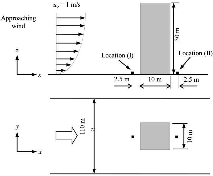
Figure 4. Geometry of wind flow around a single block and the locations of pollution sources (I) and (II), (a) front view; (b) top view.
for the turbulent energy, and turbulent intensity is assumed to be 10% of the inflow wind velocity at a representative height (zo) of 74.6 m. Free slip condition is applied to the top and side boundaries. The generalized logarithmic law with parameter E = 9 (m) is applied to building walls and the ground surface as smooth walls.
Tables 1 and 2 summarize the parameters used in the numerical simulations for both examples, together with the applied boundary conditions.
Once the flow field is solved, it is considered steady. In fact, airflow characteristics within outdoor environments are unsteady due to fluctuations in both speed and direction. However, in the present stage of this study, fluctuations in the applied wind are not considered in the analysis. Accordingly, the wind flow is treated as steady. After solving the flow field, the concentration fields in both forward-time and reverse simulations are solved against time. The wind flow distribution together with the pollutant concentrations of the forward-time simulation are used as initial conditions for the reverse simulation. A time step of ∆t = 0.1 s is used with the implicit scheme.
In forward-time simulation, a pollutant source of strength 0.01 kg/m3/s is released in the period from t = 0 to 30 s. Then, the solution of the transport equation is continued with the absence of the source until t = 100 s
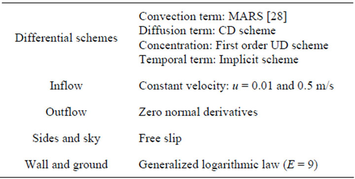
Table 1. Simulation parameters in the case of laminar flow.
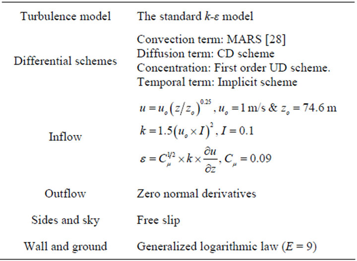
Table 2. Simulation parameters in the case of laminar flow.
for the case of laminar flow and until t = 200 s for the case of wind flow around a single building. Figure 5 shows the characteristics of the pollutant release as a function against time.
In reverse simulation, the flow field calculated by forward-time simulation is reversed at first and the source term is set to zero. Then, the transport equation is solved from the moment of t = 100 s in the reverse time direction. The time at which the reversed simulation is stopped is not known in reality. In other words, starting from the moment of solving the transport equation in the reverse time direction, the time t = 0 at which the calculations have to be stopped is not known in advance. Since the present examples are introduced just to explain the technique of direct inverse modeling, the end time is assumed.
6. Results and Discussions
6.1. Case of Laminar Flow
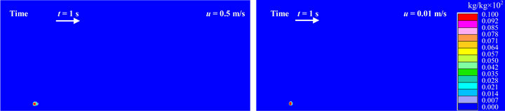
Figure 6 shows the concentration fields for two different constant inflow velocities of 0.01 and 0.5 m/s. In subplots (a) and (b), the concentration fields at t = 1 s and 100 s obtained by forward-time simulation are presented, while the subplot (c) shows the distribution of pollutant concentrations obtained through reverse simulation.
With the steady-state airflow pattern, forward-time CFD simulation was used to calculate pollutant concentration distribution at t = 100 s, where a pollution source was released from t = 0 to 30 s. The distributions of steady-state airflow and transient pollutant concentration at t = 100 s were used as initial data for the inverse CFD modeling. The inverse CFD modeling calculated backwards pollutant transport from t = 100 s to 0 s is shown in Figure 6(c).
In order to determine the pollutant release location, the distribution of pollutant concentration should be in a small region around the release source as shown in Figure 6(c), and by using the maximum pollutant concentration over all locations at this instance (the peak pollutant

Figure 5. Pollutant source strength as a function against time.
 (a)
(a)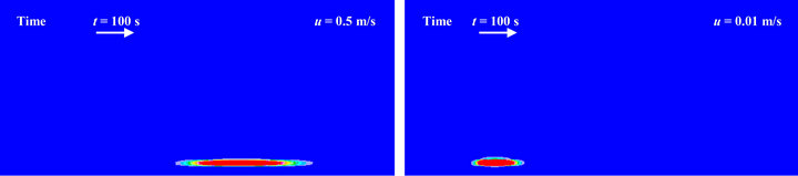 (b)
(b)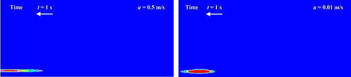 (c)
(c)
Figure 6. Concentration fields for the case of laminar flow, (a) at t = 1 s obtained by direct simulation; (b) at t = 100 s obtained by direct simulation; (c) at t = 1 s obtained by reverse simulation.
concentration), one could identify the pollution source. The peak concentration computed by inverse CFD modeling in Figure 6(c) clearly shows the position of the pollutant source.
By comparing the two concentration fields of u = 0.01 m/s and 0.5 m/s given in Figure 6(c), the case where u = 0.5 m/s shows a more dispersive concentration field compared with the case of u = 0.01 m/s. This can be attributed to the increased plume size with the increase in wind velocity. However, the direct reverse simulation appears to effectively identify the release sources in both cases.
6.2. Case of Turbulent Flow around a Single Building
Figure 7 shows the computed airflow pattern around a single building under steady state conditions. Figure 7(a) shows the flow field calculated by the forward-time simulation and Figure 7(b) shows the reversed flow field which was used to carry out the reverse simulation. In Figure 7(a), a symmetrical flow field is shown around the building, where two identical circulation regions are formed around the building.
It is expected that the effectiveness of inverse direct modeling in identifying the pollution source is affected by its location. So, as mentioned before, two locations for the pollutant source were examined here, namely locations (I) and (II). The first location is upwind of the building and the second location is in the wake region downwind of the building.
Source location (I):
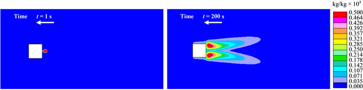
The concentration fields around the building obtained for the source at location (I) are shown in Figure 8. At t = 1, shown in Figure 8(a), the plume starts to diffuse where the concentration field makes contact with the upwind face of the building. The plume then travels with the wind downwind of the building. The pollutant continues to be released until the moment t = 30 s. At that time, the emission source was stopped and the scalar transport equation was solved against time using inverse
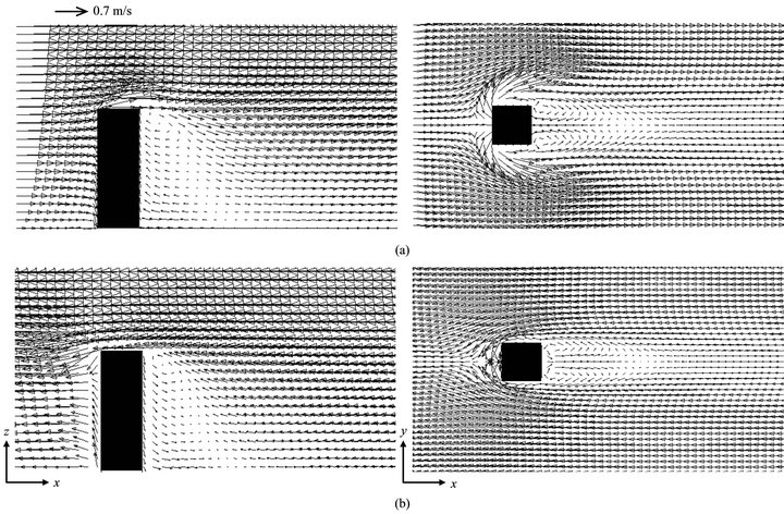
Figure 7. Wind flow field around a building, (a) direct flow field; (b) reversed flow field.
 (a)
(a)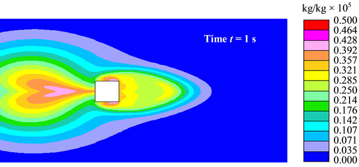 (b)
(b)
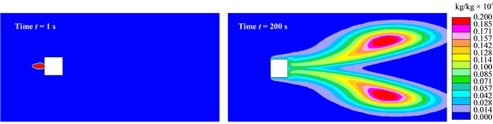
Figure 8. Concentration fields for the source is in location (I), (a) at t = 1 s obtained by forward-time simulation; (b) at t = 200 s obtained by forward-time simulation; (c) at t = 1 s obtained by reverse simulation.
direct simulation without the source. At t = 200 s, two identical regions were formed far from the building. The conditions at such time were used as the initial conditions for the inverse modeling.
Figure 8(c) shows the concentration field obtained by the inverse modeling. In such figure, the concentration field area is wider than that of the original forward-time simulation. By detecting the location of the maximum concentration overall in the domain volume, the source location is clearly determined. It is located downwind of the building along the domain centerline. However, the figure implies two problems. The first one is that the maximum concentration occupies a wide area in front of the block, which means that estimations for the location of the source will not be 100% accurate. It is thought that the wide spread of the concentration field is attributed to what is called “false diffusion”, introduced by the first order approximation of the advection term in the upwind difference scheme [29]. The second problem is that, compared to the peak concentration obtained with the forward-time simulation (see Figure 8(b)), the source strength identified by the reverse simulation (see Figure 8(c)) is more dispersive. The reason is that the reversed transport equation is not exactly the same as the governing transport equation due to the presence of a filter. Indeed, these two problems affect the prediction accuracy of the inverse modeling and this appears clearly in the wide area of the maximum concentration, which gives a wide range of possibilities for the pollution source location. This is not considered to be the ideal distribution when a gas release position is required. At the same time, the dispersive property of the reversed transport equation renders the estimated source strength inaccurate.
Source location (II):
Figure 9 shows the concentration fields around the building when the pollutant source is at location (II). Figure 9(a) shows the source location, which is 2.5 m downwind of the building’s rear wall. As with the case for location (I), the pollutant is emitted in the period from t = 0 to 30 s, and then the transport equation was solved in the absence of the source term until the moment t = 200 s. In subplot (b), two high concentration regions are formed behind the building. However, diffusion of the pollutant in this case is limited to a narrow region compared to the case for location (I).
Figure 9(c) shows the concentration field obtained using inverse modeling. The figure demonstrates that the concentration increases in the direction of the reversed wind from right to left. Also, the figure shows that the peak concentration region occupies a narrow region compared with the case for location (I). This can be attributed to the presence of the source in the wake region where a lower wind velocity exists and convection is weak. In such case, the location of the pollution source as estimated by the reverse simulation is not clear. In Figure 9(c), there are two peak concentration regions near the edges of the block. So the location of the source is not accurately identified. This indicates that the prediction
 (a)
(a)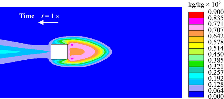 (b)
(b)
Figure 9. Concentration fields for the source is in location (II), (a) at t = 1 s obtained by forward-time simulation; (b) at t = 200 s obtained by forward-time simulation; (c) at t = 1 s obtained by reverse simulation.
accuracy of the inverse modeling is diminished in case of weak convection.
6.3. Prediction Accuracy Improvement
From the results of the above examples, it is clear that the accuracy of the method is limited due to the wide diffusion fields around the source location caused by the filter. Accordingly, a technique for improving the prediction accuracy of the method is needed. The proposed technique used what is called a “sink” in the reversed transport equation in order to decrease the widespread of the concentration field around the source and render identification of the source more easily. The reversed transport equation is then rewritten as:
 (11)
(11)
where the last term on the right-hand side is the sink term.
In order to apply the sink term technique to identify pollution source characteristics, some criteria are needed. Such criteria have to satisfy the following requirements:
• Sufficiently general to be applied to any case.
• It should show where to put the sink within the study domain.
• The criteria should give a reasonable value for the sink strength to carry out the calculations.
• Then, the following procedure is applied which couples CFD with optimization approach.
• Setting the sink at any location within the domain with any strength (S).
• Carrying out CFD simulation to solve the scalar transport equation with any release time (T)
 (12)
(12)
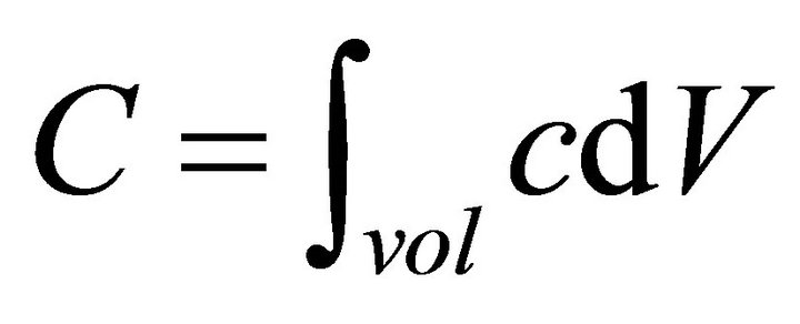
• At time (T), we calculate the whole concentration in the domain, which is:
• Then, the optimization approach is used to find the minimum value of the concentration within the domain.
• If the initial guess doesn’t give the minimum domain concentration, another trial with new sink location and new values for S and T selected by the optimization technique is used, until the minimum concentration within the domain is obtained.
A flow chart for the above mentioned procedure is shown in Figure 10.
7. Conclusions
This paper discusses the advantages and feasibility of using inverse CFD modeling to detect air pollution sources in urban environments. The study reviews vari-
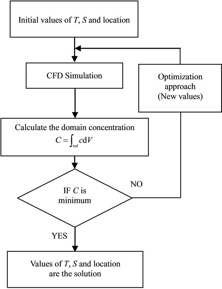
Figure 10. Flow chart of the proposed technique.
ous inverse modeling approaches and categorizes them into four techniques: the analytical technique, the optimization technique, the probabilistic technique, and the direct inverse technique. Each technique has its own advantage and limitations. The analytical approach requires analytical solution of the distributions of airflow and pollutant concentrations. However, it is only used for simple problems, which means that the applications of such technique are very limited. The optimization approach uses forward-time modeling to obtain the effectual data based on all possible causal characteristics. The limitation of this approach is that it needs a large amount of forward-time modeling. The probabilistic approach uses probability to express a possible causal aspect. In such technique all possible causal characteristics should be known before doing the modeling. The direct inverse approach solves inverse problems by reversing directly the governing equations that describe cause-effect relations. The instability problem caused by the negative diffusion term represents the main difficulty when applying such technique. The study proposed the use of a filter to account overcome the instability caused by the negative diffusion term in the scalar transport equation. In addition, in order to decrease the wide diffusion field around the source location caused by the filter, the study proposed a “sink-term” technique in the reversed transport equation to render identification of the source more easily. As a conclusion, the study reveals that the direct inverse modeling is a promising tool for detecting air pollution source in urban environments. However, more efforts are still needed to overcome the difficulties explained in the study.
REFERENCES
- K. Yokoyama, “Our Recent Experiences with Sarin Poisoning Cases in Japan and Pesticide Users with References to Some Selected Chemicals,” Neurotoxicology, Vol. 28, No. , 2007, pp. 364-373. doi:10.1016/j.neuro.2006.04.006
- T. Okumura, N. Takasu, S. Ishimatsu, S. Miyanoki, A. Mitsuhashi, K. Kumada, et al., “Report on 640 Victims of the Tokyo Subway Sarin Attack,” Annals of Emergency Medicine, Vol. 28, No. 2, 1996, pp. 129-135. doi:10.1016/S0196-0644(96)70052-5
- M. Karter, “Fire Loss in the United States during 2002,” Fire Analysis & Research Division, National Fire Protection Association, Quincy, 2003. http://www.nfpa.org/assets/files/pdf/OSfireloss02
- J. Friedr, “Stable Solution—Inverse Problems,” Vieweg & Sohn, Verlagsgesellschaft mbH, Braunschweig, 1978.
- A. Tarantola, “Inverse Problem Theory and Methods for Model Parameter Estimation,” Society for Industrial and Applied Mathematics, Philadelphia, 2004.
- O. Alifanov, “Inverse Heat Transfer Problems,” SpringerVerlag, New York, 1994. doi:10.1007/978-3-642-76436-3
- S. Alapati and Z. J. Kabala, “Recovering the Release History of a Groundwater Contaminant Using a Non-Linear Least-Squares Method,” Hydrological Processes, Vol. 14, No. 6, 2000, pp. 1003-1016. doi:10.1002/(SICI)1099-1085(20000430)14:6<1003::AID-HYP981>3.0.CO;2-W
- N. K. Ala and P. A. Domenico, “Inverse Analytical Techniques Applied to Coincident Contaminant Distributions at Otis Air Force Base, Massachusetts,” Groundwater, Vol. 30, No. 2, 1992, pp. 212-218. doi:10.1111/j.1745-6584.1992.tb01793.x
- P. Kathirgamanathan, R. Mckibbin and R. I. Mclachlan, “Source Term Estimation of Pollution from an Instantaneous Point Source,” Research Letters in Information Mathematic Science, Vol. 3, 2002, pp. 59-67.
- M. Islam and G. Roy, “A Mathematical Model in Locating an Unknown Emission Source,” Water, Air, and Soil Pollution, Vol. 136, No. 1-4, 2002, pp. 331-345. doi:10.1023/A:1015210916388
- M. Islam, “Application of a Gaussian Plume Model to Determine the Location of an Unknown Emission Source,” Water, Air, and Soil Pollution, Vol. 112, No. 3-4, 1999, pp. 241-245. doi:10.1023/A:1005047321015
- S. M. Gorelick, B. E. Evans and I. Remson, “Identifying Sources of Groundwater Pollution: An Optimization Approach,” Water Resources Research, Vol. 19, No. 3, 1983, pp. 779-790. doi:10.1029/WR019i003p00779
- B. J. Wagner, “Simultaneously Parameter Estimation and Contaminant Source Characterization for Coupled Groundwater Flow and Contaminant Transport Modeling,” Journal of Hydrology, Vol. 135, No. 1-4, 1992, pp. 275-303. doi:10.1016/0022-1694(92)90092-A
- P. S. Mahar and B. Datta, “Identification of Pollution Sources in Transient Groundwater Systems,” Water Resources Management, Vol. 14, No. 3, 2000, pp. 209-227. doi:10.1023/A:1026527901213
- A. Bagtzoglou, D. Dougherty and A. Tompson, “Application of Particle Method to Reliable Identification of Groundwater Pollution Sources,” Water Resources Management, Vol. 6, No. 1, 1992, pp. 45-23. doi:10.1007/BF00872184
- M. F. Snodgrass and P. K. Kitanidis, “A Geo-Statistical Approach to Contaminant Source Identification,” Water Resources Research, Vol. 33, No. 4, 1997, pp. 537-546. doi:10.1029/96WR03753
- M. D. Sohn, P. Reynolds, N. Singh and A. J. Gadgil, “Rapidly Locating and Characterizing Pollutant Releases in Buildings,” Journal of the Air & Waste Management Association, Vol. 52, No. 12, 2002, pp. 1422-1432. doi:10.1080/10473289.2002.10470869
- S. Kato, P. Pochanart and Y. Kajii, “Measurements of Ozone and Non-Methane Hydrocarbons at Chichi-Jima Island, a Remote Island in the Western Pacific: LongRange Transport of Polluted Air from the Pacific Rim Region,” Atmospheric Environment, Vol. 36, No. 34, 2002, pp. 385-390.
- S. Kato, P. Pochanart, J. Hirokawa, Y. Kajii, H. Akimoto, Y. Ozaki, K. Obi, T. Katsuno, D. G. Streets and N. P. Minko, “The Influence of Siberian Forest Fires on Carbon Monoxide Concentrations at Happo, Japan,” Atmospheric Environment, Vol. 36, No. 2, 2002, pp. 385-390.
- S. Kato, Y. Kajii, R. Itokazu, J. Hirokawa, S. Koda and Y. Kinjo, “Transport of Atmospheric Carbon Monoxide, Ozone, and Hydrocarbons from Chinese Coast to Okinawa Island in the Western Pacific during Winter,” Atmospheric Environment, Vol. 38, No. 19, 2004, pp. 2975-2981. doi:10.1016/j.atmosenv.2004.02.049
- J. L. Wilson and J. Liu, “Backward Tracking to Find the Source of Pollution,” Water Management Risk Remediation, Vol. 1, 1994, pp. 181-199.
- J. Ferziger and M. Peric, “Computational Methods for Fluid Dynamics,” 3rd Edition, Springer Verlag Publisher, New York, 2002. doi:10.1007/978-3-642-56026-2
- S. Patankar, “Numerical Heat Transfer and Fluid Flow,” Hemisphere Publishing Corporation, New York, 1980.
- A. C. Bagtzoglou and J. Atmadja, “Marching-Jury Backward Beam Equation and Quasi-Reversibility Methods for Hydrologic Inversion: Application to Contaminant Plume Spatial Distribution Recovery,” Water Resources Research, Vol. 39, No. 2, 2003, pp. SBH101-SBH1014. doi:10.1029/2001WR001021
- T. H. Skaggs and Z. J. Kabala, “Recovering the History of a Groundwater Contaminant Plume: Method of Quasireversibility,” Water Resources Research, Vol. 31, No. 11, 1995, pp. 2669-2673. doi:10.1029/95WR02383
- T. Zhang and Q. Chen, “Identification of Contaminant Sources in Enclosed Environments by Inverse CFD Modeling,” Indoor Air, Vol. 17, No. 3, 2007, pp. 167-177. doi:10.1111/j.1600-0668.2006.00452.x
- D. Liu, F. Zhao and H. Wanga, “History Recovery and Source Identification of Multiple Gaseous Contaminants Releasing with Thermal Effects in an Indoor Environment,” International Journal of Heat and Mass Transfer, Vol. 55, No. 1-3, 2012, pp. 422-435. doi:10.1016/j.ijheatmasstransfer.2011.09.041
- L. Bram, “Towards the Ultimate Conservative Difference Scheme, V. A Second Order Sequel to Godunov’s Method,” Journal of Computational Physics, Vol. 32, No. 1, 1979, pp. 101-136. doi:10.1016/0021-9991(79)90145-1
- T. Tsai and M. Nabil, “A Comparative Study of Central and Upwind Difference Schemes Using the Primitive Variables,” International Journal for Numerical Methods in Fluids, Vol. 3, No. 3, 1983, pp. 295-305. doi:10.1002/fld.1650030308