Journal of Financial Risk Management
Vol.3 No.2(2014), Article
ID:46719,10
pages
DOI:10.4236/jfrm.2014.32003
Continuous-Time Mean-Variance Portfolio Selection with Inflation in an Incomplete Market
Yingying Xu1, Zhuwu Wu1,2
1School of Science, China University of Mining and Technology, Xuzhou, China
2School of Management, China University of Mining and Technology, Xuzhou, China
Email: xuyy23@hotmail.com, wuzhuwu@cumt.edu.cn
Copyright © 2014 by authors and Scientific Research Publishing Inc.
This work is licensed under the Creative Commons Attribution International License (CC BY).
http://creativecommons.org/licenses/by/4.0/


Received 14 April 2014; revised 10 May 2014; accepted 3 June 2014
ABSTRACT
This paper concerns a continuous-time portfolio selection problem with inflation in an incomplete market. By using the approach of more general stochastic linear quadratic control technique (SLQ), we obtain the optimal strategy and efficient frontier to this problem. Furthermore, a numerical example is also provided.
Keywords:Portfolio Selection, Efficient Frontier, Optimal Strategy, Stochastic Linear-Quadratic Control

1. Introduction
Portfolio selection problem is a key topic in the modern finance. The seminal work of Markowitz (1952, 1959) addressed the issue of allocation of wealth in order to obtain the optimal return-risk trade-off. Since then, the mean-variance model has been extended in many aspects. Merton (1969, 1971) introduced a continuous-time model for maximizing the expected utility from investor’s consumption and terminal wealth. Zhou & Li (2000) investigated a continuous-time mean-variance portfolio problem and obtained the optimal strategy and efficient frontier by using the stochastic LQ technique, which opened up possible approach to solve the problem for more constraints. Following Zhou & Li (2000), many scholars extended this model to the more complicated market situations, such as liability, bankruptcy prohibition and incomplete market. See more details in Bielecki, Jin, Pliska, & Zhou (2005), Xie, Li, & Wang (2008) and Ji (2010).
In a real world, investors must deal realistically with the problems of inflation with the growth of economy when adopting a long-term but finite horizon investment strategy. Therefore, the consideration of inflation risk in a portfolio selection model will make it more practical. However, to our knowledge, the research on mean-variance portfolio selection under inflation is limited. The existing literature on this topic is not much as can be seen Brennan & Xia (2002) and Bensoussan, Keppo, & Sethi (2009).
The main goal of this paper is to investigate a continuous-time portfolio selection problemunder inflation in an incomplete market. It is clear that this model is more suitable and practical in most of the real-world situations, especially for long-term investors. Therefore, our focus will be on two cases. On the one hand, we investigate the incomplete market with inflation, in which there are m risky assets and one risk-free asset. The price processes of risky assets are driven by an m-dimensional Brownian motion. We also assume that the inflation factors affected by the market are random, which can be described by m + 1 Brownian motion. In general, the changes in the nominal price index are not just correlated with the risky assets’ nominal prices, but also with other uncertainties. It is reasonable that the other uncertainties can be represented by one Brownian motion, which is our (m + 1)-th Brownian motion. The original idea can be seen in Brennan & Xia (2002). On the other hand, we employ a stochastic linear quadratic (LQ) technique introduced by Zhou & Li (2000) to solve this problem. It should be pointed out that the introduction of inflation is by no means routine and does give rise to difficulties which are not encountered in Zhou & Li (2000). However, by using the more general stochastic LQ control technique in Yong & Zhou (1999), we can also obtain the optimal strategy and efficient frontier in closed forms.
The paper proceeds as follows. In Section 2, the model is formulated. Section 3 provides a closed-form solution of our model by using the more general stochastic LQ approach. Section 4 presents a numerical example. Finally, concluding remarks and suggestions for future work are given in Section 5.
2. Problem Formulation
We consider a market in which m + 1 assets are traded continuously within the time horizon . One of the assets is the risk-free whose nominal price process
  is subject to the following ordinary differential equation:
 (1)
(1)
where  is the nominal interest rate of the risk-free asset. The remaining m assets are risky and their nominal price processes
  satisfy the following stochastic differential equations:
 (2)
(2)
where  is a m-dimensional standard Brownian motion, which represents the random factors that affect risky assets’ nominal prices.
  is the appreciation rate of the ith
  risky asset, let
 .
.  is the volatility associated with the ith risky asset. Thus, the covariance matrix of risky assets is as follows:
 (3)
(3)
where the superscript “ ” represents the transpose of a vector or a matrix. As widely adopted in the literature, we assume the non-degeneracy condition of
 (4)
(4)
The nominal price of real consumption goods in the economy at time t is denoted by , which follows a diffusion process:
 (5)
(5)
where  is a (m + 1)-dimensional Brownian motion, which represents the random factors that affect the price index.
  is the expected rate of inflation, and
  is the volatility of the price index.
Remark 1. In general, the driving factors of inflation include but do not equal to the ones of the risky assets’ nominal prices. We describe randomness of the price index with , in which the foregoing m Brownian motions are the same ones that drive the risky assets’ nominal price, and the (m + 1)-th Brownian motion
  represents other randomness. Moreover, we assume that
  and
and  are independent.
Let  be a complete filtered probability space, where
  and
and
 . We assume that all the coefficient functions are continuous bounded deterministic functions on
 . We denote by
  the class of
  -valued continuous bounded deterministic functions on
 , and by
  the class of all
  -valued, progressively measurable and square integral random variables on
  under P with norm
 .
.
We denote by  the nominal wealth of the investor at time
 . Suppose the investor decides to hold
  shares of ith asset
  at time t. Then
 (6)
(6)
Let  be the total nominal market value of the ith
  asset held by the investor at time t, and let
 . We call the process
  a portfolio or a strategy of the investor.
We assume that the trading of shares takes place continuously in a self-financing fashion and there are no transaction costs or taxes. We also assume that short-selling is allowable. Then we have
 (7)
(7)
where  is the risk premium.
With the consideration of the inflation, the real value of any asset in the economy at time t is determined by deflating by the price index . The real value of the investor’s wealth is given by
 . Let
. Let . Applying Itô’s formula to
![]() , we obtain
, we obtain
 (8)
(8)
where ,
,  and
and
 .
.
Remark 2. In order to facilitate the following mathematical treatment, we give . In fact, we can also think that: it is assumed that there are m + 1 risky assets in the market, and their nominal prices are driving by m + 1 Brownian motions. The first m risky assets are the same ones we assumed before, and the (m + 1)-th risky asset is a fictitious risky asset. The ith
  risky asset’s volatility is given by the ith rank of
 . Moreover, we assume the shares of the (m + 1)-th risky asset held by the investor remains 0. Therefore, we can get
  by deriving
 .
.
The admissible strategy set under inflation with initial wealth x is defined as
 .
.
The objective of the investor is to maximize the expected terminal real wealth,  , and at the same time to minimize the variance of the terminal real wealth,
  ,
,
 .
.
This is the mean-variance model which can be expressed by the bi-objective optimization problem:
 . (9)
. (9)
It is known from Li & Ng (2000) that Equation (9) is equivalent to the following single objective optimization problem:
 , (10)
where the parameter  represents the weight imposed by the investor on the objective
 . Define
 . (11)
3. Solution to the Problem
In this section, we will apply the more general stochastic linear quadratic (LQ) control technique in Yong & Zhou (1999) to our model. Firstly, we will introduce a stochastic LQ auxiliary control problem and derive its optimal feedback control. Eventually the optimal portfolio strategy and the efficient frontier for the original mean-variance portfolio optimization problem under inflation are obtained in closed form.
3.1. Auxiliary Problem
Similar to Zhou & Li (2000), we introduce an auxiliary problem as follows:
 (12)
(12)
where . Define
 (13)
(13)
Recall Theorem 3.1 in Zhou & Li (2000) which shows the relationship between problems  and
and .
.
Theorem 1. For any , one has
 .
.
Moreover, if , then
  with
with , where
  is the wealth process corresponding to the strategy
 .
.
Let ,
, . Then Equation (8) becomes the following stochastic differential equation:
 (14)
(14)
where , and the objective function of the auxiliary problem
  becomes
 . Hence, the auxiliary problem
  is equivalent to minimizing
 (15)
(15)
Furthermore, the admissible strategy set  can be written as
 .
.
Thus the auxiliary problem  is equivalent to the following stochastic LQ control problem:
 .
.
3.2. Solution to the Auxiliary Problem
A solution of the stochastic LQ control problem  will involve, in an essential way, the following Riccati equation:
 (16)
(16)
along with the following adjoint ordinary differential equation:
 (17)
(17)
where
 ,
,
 ,
,  ,
,
 .
.
Theorem 2. Let  and
and  be the solution of Equations (16) and (17), respectively, such that
 ,
,
 .
.
Then Problem  is solvable with the optimal control being in a state feedback form,
 . (18)
Moreover, the optimal cost value is
 , (19)
where  for any matrix or vector
  and
and .
.
Proof: We first prove that the control given by Equation (18) is an admissible control. Substituting Equation (18) into Equation (14), we have
 (20)
(20)
Noting that  are continuous, and the appreciation coefficient and the diffusion coefficients are bounded continuous within t. Hence, we deduce that Equation (20) admits a unique strong solution
  which yields
 where
where  is a constant associated with the terminal time. Therefore, we have shown that
 .
.
Next, we prove that  is an optimal feedback control of state variable
![]() . For any
. For any , let
, let ![]() be the state variable associated with the control vector
be the state variable associated with the control vector . By applying Itô formula to
  and
and , and integrating them from 0 to T, taking expectations, add them together, we get
 (21)
(21)
Because
 .
.
We obtain
 and the equality holds if and only if
 ,
, . It shows that the feedback control given by Equation (18) is an optimal control and the optimal cost function can be obtained by Equation (19). The proof is completed.
 ![]()
Noting that the third constraint in Equation (16) is satisfied automatically since the assumption ,
, . Obviously, the solution of Equation (16) can be expressed by the following:
 . (22)
Let . Then noting Equation (16) and Equation (17), one has
 (23)
(23)
Since the equivalence of problem  and
and , the optimal feedback control of the auxiliary problem
  is also given by Theorem 2:
 , (24)
Substituting Equation (23) into Equation (24), we have
 .
.
3.3. Solution to the Original Problem
Let  be the wealth process under the optimal feedback control
 ![]() of the auxiliary problem
of the auxiliary problem . Substituting
  into Equation (8) yields
 (25)
(25)
Applying Itô’s formula to  yields
 (26)
(26)
Taking expectation on both side of Equations (25) and (26), which leads respectively to
 (27)
(27)
and
 (28)
(28)
The solution of Equation (27) is
 .
.
This leads to
 , (29)
where
 ,
, .
.
Similarly, by solving Equation (28) we have
 (30)
(30)
Substituting Equation (23) into Equation (30), we have

Then we get
 , (31)
where .
.
Based on the Theorem 1, if any optimal solution of problem  exists, it can be obtained by the solution
  of the auxiliary problem
  with
with . According to
 ,
,  with
with . The above two equations yield
 .
.
Thus, the optimal feedback control of the problem  can be expressed by
 with
with
 .
.
Correspondingly, the variance of the terminal wealth is
 . (32)
By substituting  and
and  into Equation (32), we have
 (33)
(33)
Substituting ,
,  and Equation (23) into Equation (33), we finally obtain the efficient frontier as follows:
 . (34)
Remark 3. If we let , and the market is complete, then Equation (34) would reduce to
 . (35)
Obviously, the result of Zhou & Li (2000) is a special case in our paper.
4. Numerical Example
In this section, we discuss a numerical example. Suppose that the market has four assets and a risk-free asset. Let’s assign the following parameters which are needed in our model: the risk-free asset , the expected value of inflation
 , the time horizon T = 2, the volatility of the price index
  , the appreciation rate of assets
  the initial wealth
 . And also suppose that the covariance matrix
  is as follows:
 .
.
After some transformations and calculations by using the above parameters, the efficient frontier of our model is obtained by the following.
 .
.
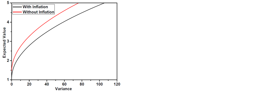
Figure 1. The efficient frontier with and without inflation.
Next, we compare our model with that of Zhou & Li (2000). The biggest difference is that our model is considered the factor of inflation in the decision-making process. Figure 1 shows the efficient frontier to continuous-time mean-variance model with and without inflation in a market. It can be seen that the frontier with inflation lies below the one without inflation. This means that the inflation plays as a penalty factor for portfolio revision. Furthermore, it tells us that the impact of it cannot be ignored in the real world when portfolio managers choose investment strategy.
5. Conclusion
This paper extends the work of Zhou & Li (2000) to an incomplete market with inflation. In our model, the inflation process is assumed to be a geometric Brownian motion, which is correlated with those of risky assets. The driving factors of inflation are not the same ones which affect risky assets’ prices. This means that the random factors affecting inflation include but do not equal to the ones of risky assets’ prices. By using the more general stochastic LQ approach, we have provided a closed-form optimal strategy and efficient frontier. Comparing to Zhou & Li (2000), our results in this paper are more general. In addition, a numerical example is also provided. There search on the liability and bankruptcy prohibition in this problem is left for future work.
Acknowledgements
We acknowledge the contributions of Fundamental Research Funds for the Central Universities (2012QNB19) and Natural Science Foundation of China (11101422, 11371362 and 71173216).
References
- Bensoussan, A., Keppo, J., & Sethi, S. P. (2009). Optimal Consumption and Portfolio Decisions with Partially Observed Real Prices. Mathematical Finance, 19, 215-236. http://dx.doi.org/10.1111/j.1467-9965.2009.00362.x
- Bielecki, T. R., Jin, H., Pliska, S. R., & Zhou, X. Y. (2005). Continuous-Time Mean-Variance Portfolio Selection with Bankruptcy Prohibition. Mathematical Finance, 15, 213-244. http://dx.doi.org/10.1111/j.0960-1627.2005.00218.x
- Brennan, M. J., & Xia, Y. (2002). Dynamic Asset Allocation under Inflation. The Journal of Finance, 57, 1201-1238. http://dx.doi.org/10.1111/1540-6261.00459
- Ji, S. (2010). Dual Method for Continuous-Time Markowitz’s Problems with Nonlinear Wealth Equations. Journal of Mathematical Analysis and Applications, 366, 90-100. http://dx.doi.org/10.1016/j.jmaa.2010.01.044
- Li, D., & Ng, W. L. (2000). Optimal Dynamic Portfolio Selection: Multiperiod Mean-Variance Formulation. Mathematical Finance, 10, 387-406. http://dx.doi.org/10.1111/1467-9965.00100
- Markowitz, H. (1952). Portfolio Selection. The Journal of Finance, 7, 77-91.
- Markowitz, H. (1959). Portfolio Selection: Efficient Diversification of Investments. New York: Wiley.
- Merton, R. C. (1969). Lifetime Portfolio Selection under Uncertainty: The Continuous-Time Case. Review of Economics and Statistics, 51, 247-257. http://dx.doi.org/10.2307/1926560
- Merton, R. C. (1971). Optimum Consumption and Portfolio Rules in a Continuous-Time Model. Journal of Economic Theory, 3, 373-413. http://dx.doi.org/10.1016/0022-0531(71)90038-X
- Xie, S., Li, Z., & Wang, S. (2008). Continuous-Time Portfolio Selection with Liability: Mean-Variance Model and Stochastic LQ Approach. Insurance: Mathematics and Economics, 42, 943-953. http://dx.doi.org/10.1016/j.insmatheco.2007.10.014
- Yong, J., & Zhou, X. Y. (1999). Stochastic Controls: Hamiltonian Systems and HJB Equations (Vol. 43). New York: Springer. http://dx.doi.org/10.1007/978-1-4612-1466-3
- Zhou, X. Y., & Li, D. (2000). Continuous-Time Mean-Variance Portfolio Selection: A Stochastic LQ Framework. Applied Mathematics and Optimization, 42, 19-33. http://dx.doi.org/10.1007/s002450010003