InfraMatics
Vol.1 No.1(2012), Article ID:20006,9 pages DOI:10.4236/inframatics.2012.11001
A Sources-of-Error Model for Acoustic/Infrasonic Yield Estimation for Above-Ground Single-Point Explosions
Los Alamos National Laboratory, Earth and Environmental Sciences, Los Alamos, New Mexico
Email: arrows@lanl.gov
Received April 1, 2012; revised May 10, 2012; accepted June 2, 2012
Keywords: Yield Estimation; Error Propagation; Seismic; Acoustic
ABSTRACT
Acoustic/infrasonic measurements contain physical information enabling an estimate of the yield of a single-point explosion that is on or above ground. A variety of semi-empirical and numerical models have been developed for estimating the yield based on the amplitude of a recorded acoustic signal. This paper utilizes existing semi-empirical models - suitable for timely yield estimation—and develops the mathematical framework to properly account for uncertainties in these models, in addition to measurement uncertainties. The inclusion of calibration parameters into our mathematical model allows for the correction of constant path specific effects that are not captured in existing semi-empirical models. The calibrated model provides a yield estimate and associated error bounds that correctly partitions total error into model error and background noise. Yield estimation with the models is demonstrated with single-point, above ground chemical explosions at Los Alamos National Laboratory (LANL) experimental testing facilities.
1. Introduction
Several empirical and semi-empirical formulations exist for predicting acoustic/infrasonic overpressure from explosions of known yield, largely for mitigating disturbances to nearby communities [1-3]. Numerical approaches also exist [4-6], but they are more time consuming and typically require detailed constraints on temperatures and winds, in addition to constraints on the ground response, before their use over simple parametric approaches is significantly advantageous. In this study, we focus on two parametric equations, the ANSI equation [1] and the BOOM equations [2], to develop expressions for maximum likelihood yield and standard error estimates from acoustic amplitudes, using an approach that partitions variance into station and model components. It is worth noting that our error model approach could be equally applied to such numerical models.
The Concept of Operations (ConOps) for this development is constrained to a single-point above-ground explosion, with known epicenter, observed by a network of acoustic sensors. The general model includes an acoustic source model with meteorological parameters that under ConOps are specified in near real-time with local meteorological sensors (for example, sensor assets at a local airport). Additionally under ConOps, path effects parameters and physical parameters in the source model are assumed known from well-designed calibration experiments. The physical model components are embedded into a probability model that partitions total variance (error) into two sources: model and noise. These components of variance are derived from the calibration experiments. This approach to yield estimation properly forms the standard error of the estimate with these two variance components, and additionally the correlation between amplitudes. Model error decreases with improvements in a source model and the best possible mathematical representation of source emplacement conditions. Both model error and noise error decrease with improvements in the representation of path effects and good physical parameter calibrations. With this formulation, correctly, only near-to-sensor incoherent noise is reduced through station averaging. This approach to yield estimation is analogous to the development for seismic identification in [7].
2. General Acoustic/Infrasonic Amplitude Model
A common mistake in error analyses is to conflate the effects of measurement error, which tend to be reduced with the addition of more measurements, and those of model error, which bias all measurements and can only be reduced through improvements in the model. One way to quantify model error is through calibration analysis, whereby well-characterized data are used to illuminate error in the model. Here, we develop general probabilistic expressions relating source yield and observed amplitude, and derive analytical expressions for the maximum likelihood yield estimate and its variance, under this framework. Notably, in Section 2.1, we describe the proper partitioning between model error and measurement error. This general model is later applied to two parametric source propagation models in Section 3.
2.1. Partitioning of Error
To first-order, an observed  amplitude,
  , (e.g. peak overpressure) from an explosion with yield
  is
is
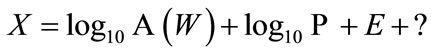 (1)
(1)
where  is the yield of the explosion.
  represents the amplitude prediction at the source (essentially the fraction of total energy that is converted into acoustic waves) and
  is the model of path effects to the sensor (incorporating various effects such as geometric spreading, non-radial expansion effects, etc.). The term
  is random model error that is common to all stations, and the term
  is a random noise variable specific to a station and near-station path. The probability model for
  is normal distributed and is generally developed in Section 2.2.
Equation (1) is a random effects linear model with model error  distributed normally with mean zero and variance
  and noise
  distributed normally with mean zero and variance
 . In this development, the stations
  have a common variance parameter
 . The random terms
  and
and  are uncorrelated, however for an explosion observed by
  stations, model error
  affects all stations making station amplitudes
  correlated (station amplitudes probabilistically move together). Observed random noise
  will be different for each station. If the physical models
  and
and  are good then
  will be small. The parameter
  can thus be considered a measure of the quality of the physical model.
2.2. Maximum Likelihood Yield Estimate and Variance
With the physical parameters in the terms  and
and  and parameters
  and
and  known through calibration, notation for the corrected log amplitude for explosion
 , station
  is
is
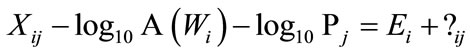 (2)
(2)
where as  is a random variable, we denote
  as the observed value of
 . Denote the vector of
  station variables
 ,
,  as
as . Then
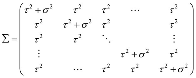
  is modeled as multivariate normal with an
  mean vector
  with elements
 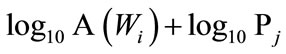 and
and  covariance matrix
 (3)
(3)
Upon substitution of observed amplitudes  (
( ), the multivariate probability density function (PDF) of
  becomes the likelihood
  used to calculate the maximum likelihood estimate (MLE)
  and associated error bounds.
With reasonable assumptions, [8-10] prove that
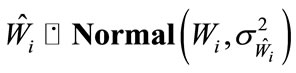 (4)
(4)
where
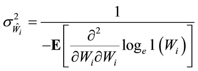 (5)
(5)
with  denoting expectation, and
  denotes “approximately distributed as”. Note that
  is generally a function of
  and this physical-basis property is correctly accounted for in Equation (5). In application
  is substituted for
  in
in .
.
For the Equation (1) model, the MLE  is the solution to the equation
 (6)
(6)
Note the change in the logarithm base due to MLE calculation with  of the multivariate normal PDF (the
  likelihood). For the Equation (1) model, direct application of Equation (5) gives
 (7)
(7)
where in application  is substituted for
 . In this general formulation, the source term
  is the same for all stations. In the following section, we review two source propagation models currently in the literature and describe their calibration. The source and path effects
  and
and  are partitioned in Section 4 to conform to the general formulation.
3. Source Model Calibration
The estimation of explosive yield requires a physical model relating observed station amplitudes to the unknown yield. Several semi-empirical source models have been developed that are analytical (readily calculated). We describe two such commonly used models below, the ANSI [1] and BOOM [2,11] models, and extend them to include simple calibration parameters. Using experimental data recorded at the LANL Seismo-Acoustic Research Center, these models are then calibrated for later yield estimation.
3.1. ANSI Model
In MKS units, the long-range ANSI distance-scaling law [1] for peak overpressure is
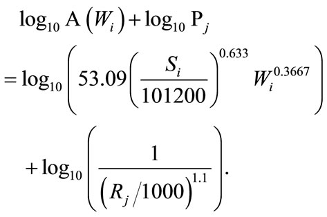 (8)
(8)
where  is the range in meters between source and the
  sensor,
  is the surface atmospheric pressure in Pascals, and
  is measured in kilograms. Note that Equation (8) is designed to compensate for inhomogeneities in the atmosphere that cause non-radial expansions. In our development we adjust Equation (8) to include path calibration parameters
  and
and  to account for source-to-sensor path effects (e.g., topographic blockage, focusing common to specific paths). These adjustments give the model
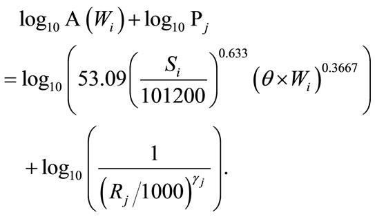 (9)
(9)
The calibrated parameters  and
and  are used in estimation calculations
  for explosions of unknown yield.
3.2. BOOM Model
The Blast Operational Overpressure Model (BOOM), developed by [11] and [2], is a semi-empirical model of broad-band peak acoustic overpressure from an explosion for range distances up to 50 kilometers that uses a single parameter  to represent the combined effect of atmospheric temperatures, and winds at a range of altitudes on air blast refraction. The BOOM model in decibels is referenced to a pressure of 20 micro-Pascals, and the model in MKS units (Pascals) is
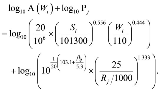 (10)
(10)
where
 .
.
In Equation (10),  is the surface atmospheric pressure in Pascals,
  has dimensions kilograms and
  is the sound speed at the surface in meters/second.
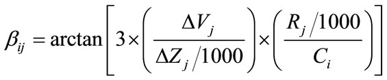
The effective sound speed (a vector sum of the isotropic sound speed, from temperature, and the wind speed in the propagation direction) relative to  varies as a function of elevation (meters) relative to the ground. There is an elevation
  where the arctangent of
  is a maximum noting that
  is the difference in the speed of sound relative to
  at elevation
 . Positive values of
  are representative of conditions that support propagation along the ground (e.g., temperature inversions), while negative values lead to increased attenuation. [2] successfully applied BOOM to two very different experimental explosion campaigns (denoted CHEBS and ISST). For CHEBS, rawinsonde observations were obtained at a distance of 10 kilometers.
  varied from 300 to 2700 meters. For ISST, rawinsonde data came from a location 40 kilometers from the source location within 30 minutes of the test time. The ISST shots had overburden which [2] successfully compensated for with an empirical correction for BOOM that accounts for known overburden—essentially
  in Equation (10) is replaced by
  for explosions with overburden.
The primary advantage of BOOM is that it allows us to incorporate knowledge of atmospheric inhomogeneities (i.e., winds and temperatures as a function of height). The required meteorological data could be readily obtained from a nearby airport radiosonde or from meteorological towers (such as used in this study), and this data would serve as an adequate approximation for the atmospheric conditions affecting propagation of acoustic/ infrasound energy from an explosion to a distant sensor. Analogous to the ANSI model formulation we adjust Equation (10) to include path calibration parameters  and
and  to account for source-to-sensor path effects. These adjustments give the model
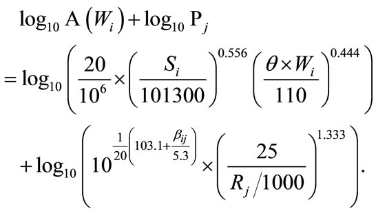 (11)
(11)
where  is defined in Equation (10). The calibrated parameters
  and
and  are used in estimation calculations
  for explosions of unknown yield.
3.3. Calibration
The LANL Seismo-Acoustic Research Center (SARC) is a collaboration between the LANL Geophysics group and the LANL Weapons Experiments group (WX). In this paper, we report on 14 single-charge explosions and measured peak overpressure amplitudes from acoustic waveforms at five stations, used to calibrate the previously described models. Figure 1 shows the topography around the SARC experiment sites Minie and Lower Slobovia, and the locations of the 5 sensor sites DetMoe, TA46, TA51 and sensor station TT in the community of White Rock, New Mexico. SARC/WX explosion experiments are executed regularly (several times per week) and with a diversity of yields and emplacement conditions. Meteorological data for these experiments (wind speed and direction, and temperature from various heights up to 100 meters above ground-level, as well as ambient atmospheric pressure measurements) was acquired from the LANL TA-06 meteorological tower. Data from these experiments are provided in the Appendix.
As discussed above, parameter calibration analysis is demonstrated with SARC explosions with yields significantly less than 181 kilograms to obtain calibrated (estimated) values for  and
and . Event 12 in the Appendix, with a yield of 181 kilograms, was left out of the calibration study in order to later assess how well a much larger shot can be estimated given the calibration results for smaller explosions. We adopt a 2-stage calibration procedure to utilize existing software. For the first stage, least squares is a reasonable and easily implemented objective function for calibrating the parameters
  and
and
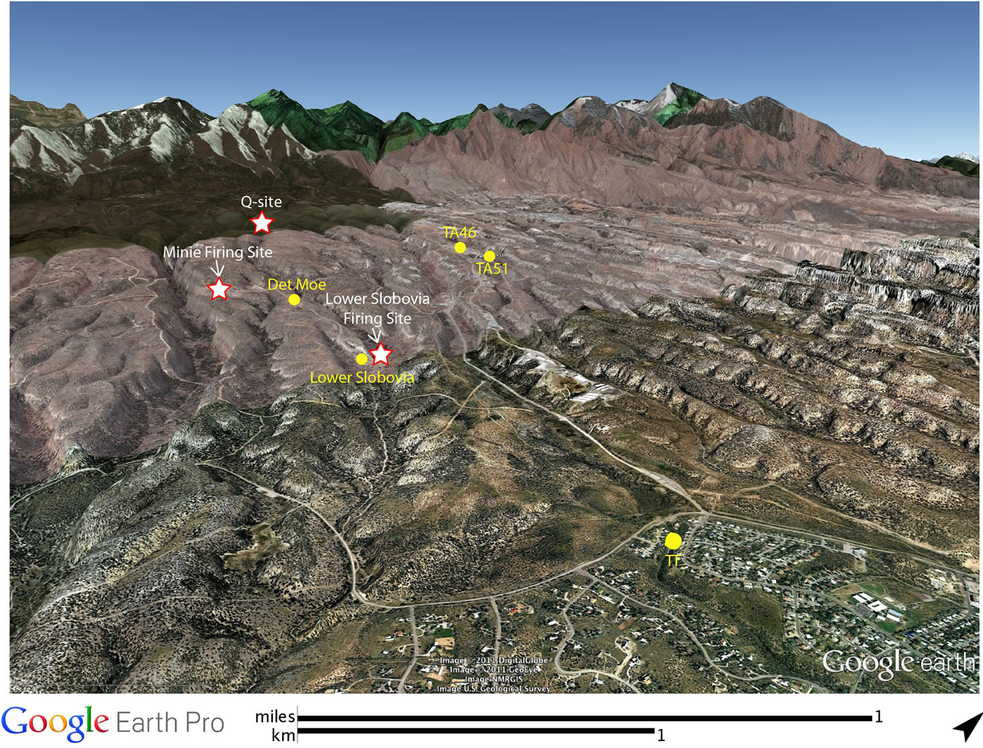
Figure 1. Map showing the locations of WX firing sites for shots analyzed in this study (white stars) and locations of seismoacoustic sensor systems (yellow circles). We note that the station at Lower Slobovia is not used in this study. The study region is characterized by a series of canyons and mesas, introducing topographic effects that are unique to each shot-sensor path.
 . Specifically, for the
  calibration explosions, minimizing
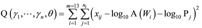 (12)
(12)
gives calibration values  and
and  for the ANSI and BOOM models respectively. These values are provided in Table 1. Analogous to the left side of Equation (2), substituting the respective calibration values into the BOOM source model gives the fit residuals
 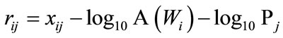 (
( for the ANSI model) and these residuals can then be used to calibrate the parameters
  and
and  with a standard oneway random effects model
 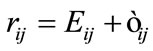 (see [12]). We perform two separate calibration studies: 1) using all explosions recorded by the stations Det Moe and Tom Turner, and 2) using only those explosions recorded by Det Moe and Tom Turner associated with an atmospheric profile refracting the sound waves upward (i.e., negative
  values). We note that observations at stations TA46 and TA51, which are located across several canyons and mesas from the explosion sites, are not well predicted by either model. We speculate that topographic effects, which are not accounted for in this study, cause the poor predictions to TA46 and TA51; the calibration parameters
  do not adequately correct for the complex interplay of topography and atmospheric effects along these paths. Further analysis of topographic effects is a key recommendation for future research. Calibration values for
  and
and  for both scenarios are given in Table 1, and summary comparisons of the fit of the two models are given in Figure 2.
4. Demonstrated Yield Estimation
We use the calibrated ANSI and BOOM models to estimate the yield of a known test explosion from observed acoustic amplitudes (Table 2, ID 12), and produce associated confidence intervals from our analytical expression for partitioned variance, Equation (7). The test event had a yield of 181 kilograms and was observed at two stations, DetMoe and TT, 940 meters and 5380 meters away, respectively. For the ANSI model, the maximum likelihood estimate Equation (6) gave  for
for
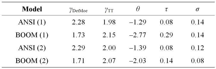
Table 1. Calibrated parameter values for ANSI and BOOM models for scenarios (1) and (2) in the text.
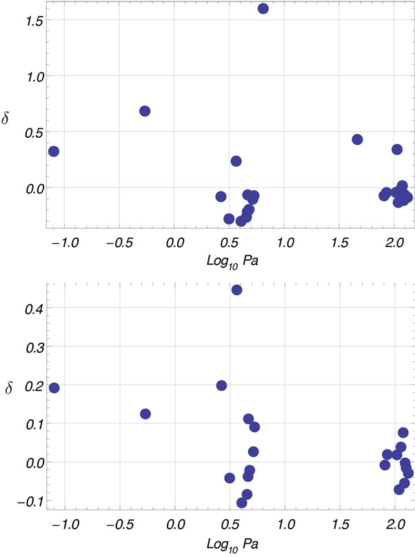
Figure 2. Plots of 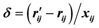 versus xij (observed log10 amplitude) for scenario 1 (top) and scenario 2 (bottom). Positive values indicate that the BOOM model provides a better fit to the calibration explosions.
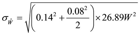
scenario 1 and  for scenario 2. For scenario 2, Equation (7) calculations give the following standard error for the ANSI model:
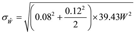 (13)
(13)
Substituting the MLE  for
for  gives an estimated standard error of
  (which is
  for scenario 1) For the BOOM model, the maximum likelihood estimate Equation (6) gave
  for scenario 1 and
  for scenario 2. For scenario 2, Equation (7) calculations give the following standard error for the BOOM model:
 (14)
(14)
Substituting the MLE  for
for  gives an estimated standard error of
  (or
(or  for scenario 1). For general values of
 , the standard errors for the two models (represented by Equations (13) and (14) for scenario 2) are given in Figure 3.
For the dataset presented in this paper, our results suggest that the BOOM model, calibrated for smaller shots, provides improved predictions for a single larger shot when the effective sound speed profile causes sound

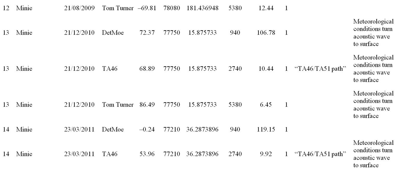
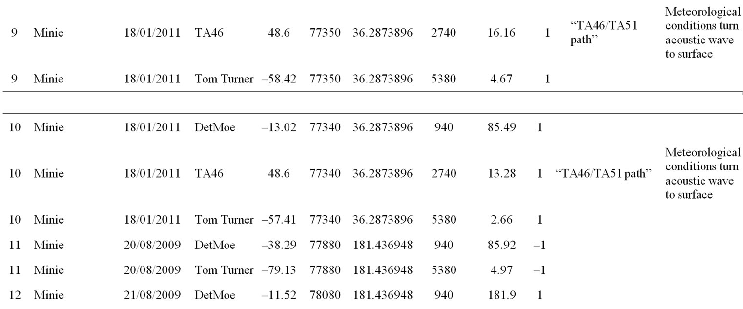
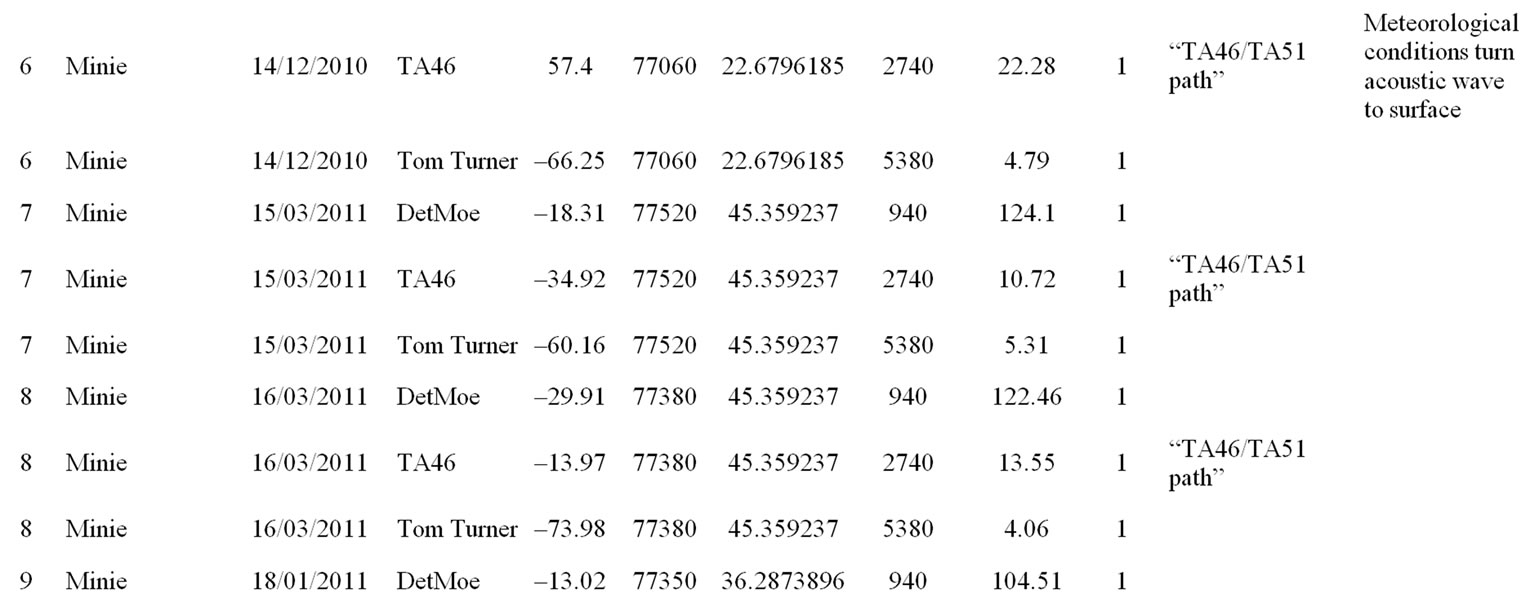
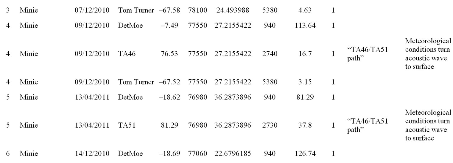
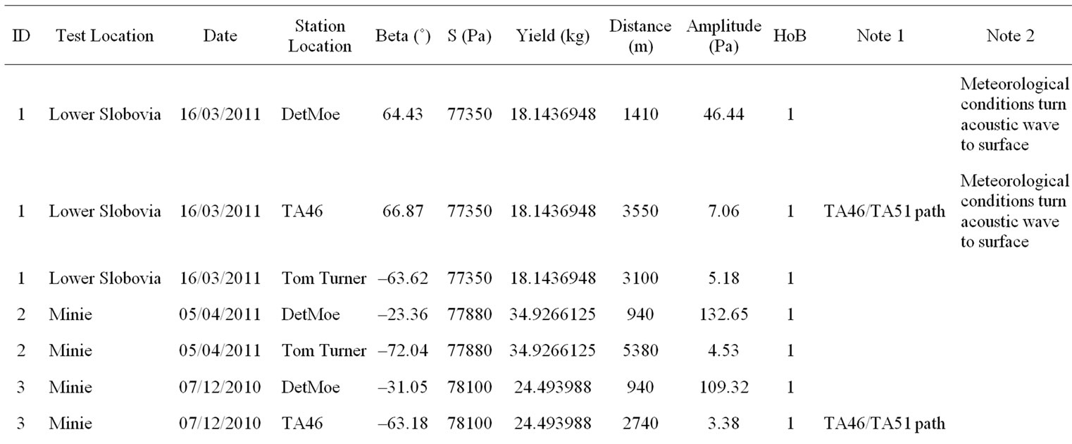
Table 2. SARC acoustic overpressure amplitudes, meteorological measurements and height of burst (HoB). The Height of burst column contains a set of flags that indicate whether the shot is on or above the ground (1) or buried (0).
to be refracted upwards, whereas ANSI performs better when sound is refracted towards the ground. We note that the values of  used in [4] are most commonly negative or slightly positive; most blasting typically occurs when sound is expected to be refracted upwards, minimizing disturbances to communities. Our results imply the need to re-evaluate the BOOM equations for cases where sound is strongly refracted towards the ground.
For scenario 2, suppose both the ANSI and BOOM models gave estimated yields equal to the true yield. Then the estimated standard errors for both the ANSI and BOOM yield estimates would be 138.8 kg. The test conditions for the SARC/WX experiments were very similar giving comparable model error components  for both models. It is reasonable to expect that
  would increase for calibration experiments from diverse, and importantly, unknown emplacement conditions. This leads to the conclusion that the best initial strategy to reduce the standard error of a yield estimate is to improve path effects models, primarily reducing
 .
.
Application of the variance-partitioning framework presented here demonstrates that improved physical path models should be high priority in improving the yield estimation model Equation (1). Through the random effects formulation, we are able to explicitly attribute higher confidence in the estimate to improvements in a physical path model. Of equally high priority is the realistic specification of model error  to include unknown emplacement conditions. The specification of
  should include understanding acquired from realistic calibration experiments from a diversity of emplacement conditions.
5. Summary and Future Developments
We have developed expressions for maximum likelihood yield and standard error estimates for the general yield
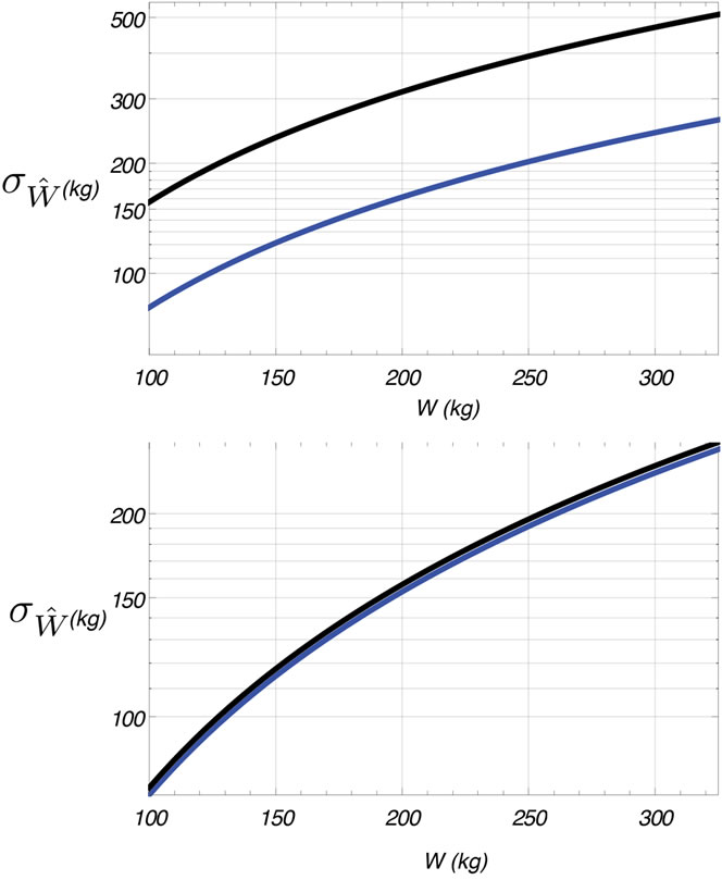
Figure 3. Standard error of a yield estimate Ŵ for the BOOM (black) and ANSI (blue) source models with n = 2 for scenario 1 (top) and scenario 2 (bottom).
estimation model Equation (1), and specifically we have correctly partitioned model and measurement error in the standard error equation. We have demonstrated this framework with two calibrated source propagation models, the ANSI [1] and BOOM models [2,11]. Calibration of error components was demonstrated, as was yield estimation demonstrated using a 181-kilogram test explosion. The BOOM model produces a more accurate yield estimate, with correspondingly smaller variance, for the unknown explosion, but only once measurements made when sound is refracted downwards are removed. The ANSI model is more robust over all possible atmospheric scenarios.
From the discussion in Section 4, our future analytical research will center on the development of more sophisticated analytical acoustic path correction models, and equally important the development of an analytical maximum likelihood framework for seismic/acoustic/infrasonic (seismo-acoustic) yield estimation. The development of acoustic path models will explore the correction for topographic effects using data from stations at TA46 and TA51; previous studies have modeled topographic effects on explosion signals using a series of finite sized barriers [13]. We also plan to incorporate 3D (range dependent) atmospheric effects by utilizing meteorological measurements from multiple spatial locations, and to explore models for ground impedance effects. We intend to explore simple corrections for expected sound refractions that are applicable over all atmospheric conditions. We will continue to apply the developed theory to calibration explosions with diverse emplacement conditions to better understand the specification of . Finally, we note that the mathematical framework developed in this paper can equally be applied to the assessment of the model error associated with long-range infrasound attenuation relations [14,15]. Such relations should be assessed with a comprehensive set of ground-truth events.
6. Acknowledgements
We thank David Green and Alexis Le Pichon for their thoughtful comments on an earlier version of this paper. The authors acknowledge the support of Dr. Thomas E. Kiess and the National Nuclear Security Administration Office of Nonproliferation and Treaty Verification Research and Development for funding this work. Los Alamos National Laboratory completed this work under the auspices of the U.S. Department of Energy under contract DE-AC52-06NA24596. The authors also acknowledge the support of Dr. Phillip J. Cole and the Defense Threat Reduction Agency for funding this work.
REFERENCES
- ANSI, “Estimating Airblast Characteristics for Single Point Explosions in Air, With a Guide to Evaluation of Atmospheric Propagation and Effects,” Technical report, 1983.
- D. A. Douglas, “Blast Operational Overpressure Model (BOOM): An Airblast Prediction Method,” Technical report, Air Force Weapons Laboratory, Kirtland AFB, NM, 1987.
- M. J. McFarland, J. W. Watkins, M. M. Kordich, D. A. Pollet and G. R. Palmer, “Use of Noise Attenuation Modeling in Managing Missile Motor Detonation Activities,” Journal of the Air and Waste Management Association, Vol. 54, No. 3, 2004, pp. 342-351. doi:10.1080/10473289.2004.10470909
- L. R. Hole, “An Experimental and Theoretical Study of Propagation of Acoustic Pulses in a Strongly Refracting Atmosphere,” Applied Acoustics, Vol. 53, No. 1-3, 1998, pp. 77-94. doi:10.1016/S0003-682X(97)00039-X
- C. Madshus, F. Lovholt, A. Kaynia, L. R. Hole, K. Attenborough and S. Taherzadeh, “Air-Ground Interaction in Long Range Propagation of Low Frequency Sound and Vibration-Field Tests and Model Verification,” Applied Acoustics, Vol. 66, No. 5, 2005, pp. 553-578. doi:10.1016/j.apacoust.2004.09.006
- E. M. Salomons, “Computational Atmospheric Acoustics,” 1st Edition, Kluwer Academic Publishers, Berlin, 2001. doi:10.1007/978-94-010-0660-6
- D. N. Anderson, W. R. Walter, D. K. Fagan, T. M. Mercier and S. R. Taylor, “Regional Multi-Station Discriminants: Magnitude, Distance and Amplitude Corrections and Sources of Error,” Bulletin of the Seismological Society of America, Vol. 99, No. 2A, 2009, pp. 794-808. doi:10.1785/0120080014
- M. J. Crowder, “Maximum Likelihood Estimation for Dependent Observations,” Journal of the Royal Statistical Society (B), Vol. 38, No. 1, 1976, pp. 45-53.
- R. D. H. Heijmans and J. R. Magnus, “Consistent Maximum Likelihood Estimation with Dependent Observations: The General (Non-Normal) and the Normal Case,” Journal of Econometrics, Vol. 32, No. 2, 1986, pp. 253- 285. doi:10.1016/0304-4076(86)90040-0
- Y. R. Sarma, “Asymptotic Properties of Maximum Likelihood Estimators from Dependent Observations,” Statistics & Probability Letters, Vol. 4, No. 6, 1986, pp. 309- 311. doi:10.1016/0167-7152(86)90050-7
- R. A. Lorentz, “Noise Abatement Investigation for the Bloodsworth Island Target Range: Description of the Test program and New Long Range Airblast Overpressure Prediction Method,” Technical Report, Naval Surface Weapons Center, Silver Springs, MD, 1981.
- D. C. Montgomery, “Design and Analysis of Experiments,” John Wiley & Sons, New York, 1984.
- D. J. Saunders and R. D. Ford, “A Study of the Reduction of Explosive Impulses by Finite Sized Barriers,” Journal of the Acoustical Society of America, Vol. 94, No. 5, 1993, pp. 2859-2875. doi:10.1121/1.407343
- R. Whitaker and P. Mutschlecner, “A Comparison of Infrasound Signals Refracted from Stratospheric and Thermospheric Altitudes,” Journal of Geophysical Research, Vol. 113, 2008, Article ID: D08117, 13 p.
- A. Le Pichon, L. Ceranna and J. Vergoz, “Incorporating Numerical Modeling into Estimates of the Detection Capability of the IMS Infrasound Network,” Journal of Geophysical Research, Vol. 117, 2012, Article ID: D05121, 12 p.