ABSTRACT

The purpose of this study was to demonstrate a simple and fast method for solving the time-dependent Bloch-McConnell equations describing the behavior of magnetization in magnetic resonance imaging (MRI) in the presence of multiple chemical exchange pools. First, the time-dependent Bloch- McConnell equations were reduced to a homogeneous linear differential equation, and then a simple equation was derived to solve it using a matrix operation and Kronecker tensor product. From these solutions, the longitudinal relaxation rate (R_1ρ) and transverse relaxation rate in the rotating frame (R_2ρ) and Z-spectra were obtained. As illustrative examples, the numerical solutions for linear and star-type three-pool chemical exchange models and linear, star- type, and kite-type four-pool chemical exchange models were presented. The effects of saturation time (ST) and radiofrequency irradiation power (ω₁) on the chemical exchange saturation transfer (CEST) effect in these models were also investigated. Although R_1ρ and R_2ρ were not affected by the ST, the CEST effect observed in the Z-spectra increased and saturated with increasing ST. When ω₁ was varied, the CEST effect increased with increasing ω₁ in R_1ρ, R_2ρ, and Z-spectra. When ω₁ was large, however, the spillover effect due to the direct saturation of bulk water protons also increased, suggesting that these parameters must be determined in consideration of both the CEST and spillover effects. Our method will be useful for analyzing the complex CEST contrast mechanism and for investigating the optimal conditions for CEST MRI in the presence of multiple chemical exchange pools.

Keywords:

Bloch-McConnell Equations, Multiple Chemical Exchange Pools, Chemical Exchange Saturation Transfer (CEST) Magnetic Resonance Imaging (MRI), Amide Proton Transfer (APT) MRI, Numerical Analysis

1. Introduction

Chemical exchange saturation transfer (CEST) is a novel contrast mechanism for magnetic resonance imaging (MRI) [1] and has been increasingly used to detect dilute proteins via the interaction between labile solute protons and bulk water protons [2] [3] [4] . Moreover, amide proton transfer (APT) imaging, a particular type of CEST MRI that specifically probes labile amide protons of endogenous mobile proteins and peptides in tissue, has been explored for imaging diseases such as acute stroke and tumor, and is currently under intensive evaluation for clinical translation [5] [6] . Furthermore, various CEST agents have been actively developed to detect the parameters that reflect tissue pH and molecular environment and/or to enhance the CEST effect [7] . However, CEST or APT MRI contrast mechanism is complex, depending on not only the concentration of CEST agents or amide protons, exchange and relaxation properties, but also varying with experimental conditions such as magnetic field strength and radiofrequency (RF) power [8] . When there are multiple exchangeable sites within a single CEST system, the CEST contrast mechanism becomes even more complex [9] . Thus, in analyzing the complex CEST contrast mechanism and for investigating the optimal study conditions, numerical simulations are useful and effective [10] [11] . To perform extensive numerical simulations for CEST or APT MRI, it will be necessary to develop a simple and fast method for obtaining the numerical solutions to the time-dependent Bloch-McConnell equations.

The purpose of this study was to present a simple and fast method for solving the time-dependent Bloch-McConnell equations for analyzing the behavior of magnetization in MRI in the presence of multiple chemical exchange pools.

2. Materials and Methods

2.1. Bloch-McConnell Equations in a Two-Pool Chemical Exchange Model

Figure 1 illustrates a two-pool chemical exchange model in which pool A re- presents the bulk water pool. The time-dependent Bloch-McConnell equations in the two-pool exchange model for CEST MRI are given by [10] [11]

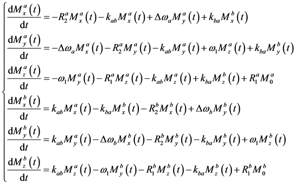, (1)

where superscripts a and b show the parameters in pool A and pool B, respectively. For example, , , and denote the x, y, and z components of the magnetization in the rotating frame in pool A at time t, respectively. and denote the longitudinal and transverse relaxation rates, i.e., the reciprocals of the longitudinal and transverse relaxation times in pool A, respectively. denotes the exchange rate from spins in pool A to those in pool B, whereas denotes that from spins in pool B to those in pool A. and denote the thermal equilibrium z magnetizations in pool A and pool B, respectively. and are given by and, respectively, where and are the Larmor frequencies in pool A and pool B, respectively, and is the frequency of the RF irradiation applied along the x axis of the rotating frame. ω₁ is the amplitude of the RF irradiation.

The differential equations given by Equation (1) can be combined into one vector equation (homogeneous linear differential equation) [11] :

, (2)

where

(3)

and

, (4)

where T in Equation (3) denotes the matrix transpose. According to Koss et al. [12] , the matrix A can be given by

, (5)

where E is the evolution matrix [12] and C is the constant-term matrix. Furthermore, E is given by

. (6)

In the case of A given by Equation (4), R is reduced to

, (7)

where

(8)

and

. (9)

K in Equation (6) is given by

, (10)

where I is a 3-by-3 identity matrix and denotes the Kronecker tensor product. C in Equation (5) is given by

. (11)

The solution of Equation (2) can be given by [11]

, (12)

where t represents the so-called saturation time and is the matrix of initial values at. is the matrix exponential.

2.2. Linear Three-Pool Chemical Exchange Model

Figure 2(a) illustrates a linear three-pool chemical exchange model in which pool A represents the bulk water pool. In this case, R and K are given by [12]

(13)

and

, (14)

respectively. in Equation (13) is given by Equation (8) in which the subscript a and superscript a are replaced by c. C is given by

. (15)

2.3. Triangular Three-Pool Chemical Exchange Model

Figure 2(b) illustrates a triangular three-pool chemical exchange model in which pool A represents the bulk water pool. In this case, K is given by [12]

. (16)

2.4. Linear Four-Pool Chemical Exchange Model

Figure 3(a) illustrates a linear four-pool chemical exchange model in which pool A represents the bulk water pool. In this case, R and K are given by [12]

(17)

and

, (18)

respectively. R^d in Equation (17) is given by Equation (8) in which the subscript a and superscript a are replaced by d. C is given by

. (19)

2.5. Star-Type Four-Pool Chemical Exchange Model

Figure 3(b) illustrates a star-type four-pool chemical exchange model in which pool A represents the bulk water pool. In this case, K is given by [12] .

. (20)

2.6. Kite-Type Four-Pool Chemical Exchange Model

Figure 3(c) illustrates a kite-type four-pool chemical exchange model in which pool A represents the bulk water pool. Although there are no chemical exchanges between pool C and pool D in the star-type four-pool chemical exchange model (Figure 3(b)), there are exchanges between them in the kite-type model (Figure 3(c)). In this case, K is given by [12]

. (21)

It should be noted that mass balance imposes the following relationship between the exchange rates and of pool I and pool J [10] :

(22)

and

(23)

2.7. Calculation of R_1ρ, R_2ρ, and Z-Spectra

The longitudinal relaxation rate in the rotating frame was obtained from the negative of the largest (least negative) real eigenvalue of the matrix A in Equation (2), i.e., [12] [13] .

The transverse relaxation rate in the rotating frame was obtained from the absolute value of the largest real part of the complex eigenvalue of the matrix A in Equation (2), i.e., [13] .

The CEST effect has usually been analyzed using the so-called Z-spectrum [11] . Thus, we calculated the Z-spectrum by using the following equation:

, (24)

where denotes the z magnetization of pool A (bulk water) with saturation at. It should be noted that is the offset frequency of the RF irradiation from the Larmor frequency of bulk water protons, i.e., . In this study, was varied from −3000 Hz to 3000 Hz with an interval of 100 Hz.

2.8. Simulation Studies

Because we have already treated a two-pool chemical exchange model in our previous paper [11] , we treated three-pool and four-pool chemical exchange models in this study.

First, we considered the three-pool exchange model consisting of bulk water (pool A) and two labile proton pools (pool B and pool C) as illustrative examples. In this case, we assumed that the longitudinal and transverse relaxation times for bulk water were 3 s and 100 ms, respectively, and were 1 s and 15 ms for two labile protons, i.e., and [9] . The chemical shifts for two labile protons were set to be 4 ppm and 5 ppm. It should be noted that the chemical shifts of 4 ppm and 5 ppm correspond to of 1192.8 Hz and 1491.0 Hz, respectively, for the magnetic field strength of 7 T. Unless specifically stated, , , and were assumed to be 100 Hz, 300 Hz, and 100 Hz, respectively., , and were assumed to be 1, 1/250, and 1/500, respectively. The saturation time and were taken as 5 s and 50 Hz, respectively.

For four-pool exchange models, we simulated one nuclear Overhauser effect site (pool D) in addition to the above bulk water (pool A) and two labile proton pools (pool B and pool C). We assumed that the longitudinal and transverse relaxation times for pool D were 1 s and 5 ms, respectively [9] . The chemical shift for pool D was set to be −3.5 ppm. It should be noted that the chemical shift of −3.5 ppm corresponds to of −1043.7 Hz for the magnetic field strength of 7 T. Unless specifically stated, and were assumed to be 10 Hz and 10 Hz, respectively. was assumed to be 1/500.

Calculations were performed using MATLAB® (The MathWorks Inc., Natick, MA, USA) on an Intel Core^TM i7-4790 CPU (3.6 GHz) with 8-GB RAM. The matrix exponential and Kronecker tensor product were calculated using the MATLAB® functions “expm” and “kron”, respectively.

3. Results

Figure 4 shows the (a), (b), and Z-spectra (c) as a function of offset frequency for various saturation times (0.5, 1, 2, 5, and 10 s) in the linear three-pool chemical exchange model (Figure 2(a)). It should be noted that the common logarithm of the value was plotted in Figure 4(a) in order to enlarge the change in the value. The peaks at 0 Hz (0 ppm), 1192.8 Hz (4 ppm), and 1491.0 Hz (5 ppm) derive from pool A, pool B, and pool C, respectively. As shown in Figure 4, and were not affected by the saturation time, whereas Z-spectra changed largely depending on the saturation time, i.e., Z-spectra became broad and tended to saturate with increasing saturation time.

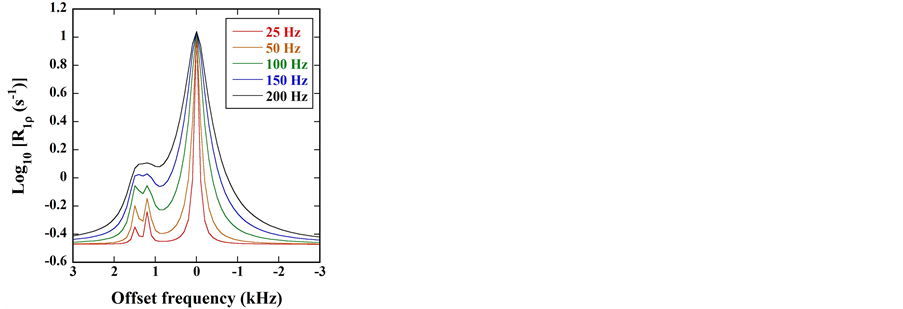
Figure 5 shows the (a), (b), and Z-spectra (c) as a function of for various values (25, 50, 100, 150, and 200 Hz) in the linear three- pool chemical exchange model (Figure 2(a)). As in Figure 4, the peaks at 0 Hz (0 ppm), 1192.8 Hz (4 ppm), and 1491.0 Hz (5 ppm) derive from pool A, pool B, and pool C, respectively. As shown in Figure 5, all parameters became broad with increasing value.

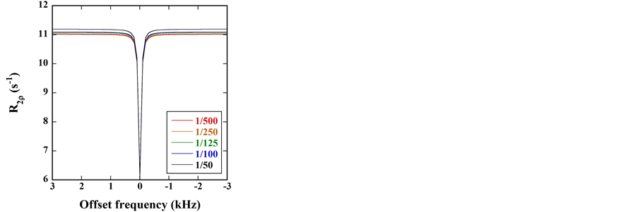
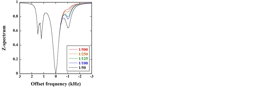
Figure 6 shows the (a), (b), and Z-spectra (c) as a function of for various values (1/500, 1/250, 1/125, 1/100, and 1/50) in the triangular three-pool chemical exchange model (Figure 2(b)). As shown in Figure 6(a) and Figure 6(c), the peaks at 1491.0 Hz (5 ppm) derived from pool C changed largely depending on in both and Z-spectra. The peaks at 1192.8 Hz (4 ppm) derived from pool B also changed but to a lesser extent. As shown in Figure 6(b), the values increased with increasing value.

Figure 7 shows the (a), (b), and Z-spectra (c) as a function of for various values (25, 50, 100, 150, and 200 Hz) in the linear four- pool chemical exchange model (Figure 3(a)). When was small, four peaks were clearly observed at 0 Hz (0 ppm), 1192.8 Hz (4 ppm), 1491.0 Hz (5 ppm),

and −1043.7 Hz (−3.5 ppm) in the and Z-spectrum plots. Note that these peaks derive from pool A, pool B, pool C, and pool D, respectively. The distinct separation among these peaks degraded with increasing value.

Figure 8 shows the (a), (b), and Z-spectra (c) as a function of for various values (1/500, 1/250, 1/125, 1/100, and 1/50) in the star-type four-pool chemical exchange model (Figure 3(b)). As in Figure 7, the peaks at 0 Hz (0 ppm), 1192.8 Hz (4 ppm), 1491.0 Hz (5 ppm), and −1043.7 Hz (−3.5 ppm) derive from pool A, pool B, pool C, and pool D, respectively. As shown in Figure 8(a) and Figure 8(c), the peaks of and Z-spectra at −1043.7 Hz (−3.5 ppm) derived from pool D changed depending on the value. The values slightly increased with increasing value (Figure 8(b)).

Figure 9 shows the (a), (b), and Z-spectra (c) as a function of for various values (10, 100, 200, 500, and 1000 Hz) in the kite- type four-pool chemical exchange model (Figure 3(c)). As in Figure 7 and Figure 8, the peaks at 0 Hz (0 ppm), 1192.8 Hz (4 ppm), 1491.0 Hz (5 ppm), and −1043.7 Hz (−3.5 ppm) correspond to pool A, pool B, pool C, and pool D, respectively. As shown in Figure 9(a) and Figure 9(c), the peaks of and Z-spectra at −1043.7 Hz (−3.5 ppm) changed depending on the value. The peaks at 1491.0 Hz (5 ppm) derived from pool C also changed but to a lesser extent. The value did not change depending on the value (Figure 9(c)).

4. Discussion

In this study, we developed a simple equation for solving the time-dependent

Bloch-McConnell equations in the presence of multiple chemical exchange pools by combining our previous method [11] and the approach presented by Koss et al. [12] . As described in our previous paper [11] , the numerical solutions obtained by our method agreed with the analytical solutions given by Mulkern and Williams [14] . We also compared the solutions obtained by our method for the two-pool exchange model with those obtained using a fourth/fifth-order Runge- Kutta-Fehlberg (RKF) algorithm and found that there was a good agreement between them [11] . These results appear to indicate the validity of our method. Furthermore, the computation time was considerably reduced when using our method (by a factor of approximately 2500 compared to the case when using the RKF algorithm [11] ). Thus, our method can be included in the nonlinear least- squares fitting routine to calculate parameters such as the exchange rate or lifetime of CEST agents [10] .

For calculating the solutions to the time-dependent Bloch-McConnell equations using Equation (12), most computation time is spent calculating the eigenvectors and eigenvalues of matrix A. However, it is necessary to carry out this calculation only once regardless of t in Equation (12). As previously described, in this study, the matrix exponential was computed using the MATLAB^® function “expm”, in which a scaling and squaring algorithm with Pade approximation [15] has been used.

In our previous study [11] , we used the two-pool exchange model for CEST or APT MRI as an illustrative example. As pointed out by Woessner et al. [10] , paramagnetic CEST agents often have more than one type of exchangeable proton. For such cases, it is necessary to expand the Bloch-McConnell equations to multi-pool exchange models. Recently, Koss et al. [12] presented a generalized expression for the evolution matrix in the Bloch-McConnell equations in the presence of multiple chemical exchange sites. In their method, the Kronecker tensor product was used [12] . As shown in this study, our method could be easily extended to multi-pool chemical exchange models by modifying matrix A in Equation (12) with use of their approach.

As previously described, was obtained from the negative of the largest (least negative) real eigenvalue of matrix A in Equation (2). was obtained from the absolute value of the largest real part of the complex eigenvalue of matrix A in Equation (2). We previously compared the and values thus obtained with those obtained numerically and found that there was a good agreement between them [13] , indicating the validity of these procedures.

The spectral dependence of CEST is determined by sweeping the RF irradiation frequency while monitoring the water resonance [1] . As previously described, the CEST effect has usually been analyzed using the so-called Z-spectrum [11] . The Z-spectrum is obtained by plotting the z component of the magnetization of pool A, i.e., bulk water proton in the form of versus irradiation offset frequency (Equation (24)). As shown in Figure 4(a) and Figure 4(b), and were not affected by the saturation time, because the matrix A in Equation (2) is independent of the saturation time. On the other hand, the Z-spectra were affected by the saturation time, i.e., the CEST effect observed in the Z-spectra increased and saturated with increasing saturation time (Figure 4(c)). When the RF irradiation power was varied, the CEST effect increased with increasing in, , and Z-spectra (Figure 5 and Figure 7). When is large, however, its saturation bandwidth is broad and thus may directly saturate the bulk water, causing the so-called spillover effect [8] . As shown in Figure 5 and Figure 7, the separation among peaks in the and Z-spectrum plots degraded with increasing, which appears to be due to the spillover effect. These results suggest that must be determined in consideration of both the CEST effect and the spillover effect. Simulation studies with use of our method will be useful especially in such a case.

As shown in Figure 6(b) and Figure 8(b), the values increased with increasing or value. When or increased, the interaction between bulk water protons and protons in pool C or pool D would increase, leading to an increase of. Our previous study demonstrated that the value increased with increasing value in a two-pool chemical exchange model [13] . This would also be applicable to the case of multi-pool chemical exchange models. Thus, the above finding would be able to be explained by the fact that the value increases with increasing or value.

Recently, Koss et al. [12] presented analytical expressions for in the presence of multiple chemical exchange sites and pointed out that analytical solutions facilitate understanding of the relationship between model parameters and the phenomenological relaxation rate constant and can lead to new methodological advances. Numerical solutions also appear to be useful for optimizing parameters such as the saturation time and for acquiring CEST or APT MRI data, because they can be easily obtained under various and/or complex study conditions in which analytical solutions may not always be obtained.

5. Conclusion

We presented a simple and fast numerical method for solving the time-dependent Bloch-McConnell equations in the presence of multiple chemical exchange pools by combining our previous method [11] and the approach presented by Koss et al. [12] . The present method will be useful for analyzing the complex CEST contrast mechanism and for investigating the optimal conditions for CEST MRI in the presence of multiple chemical exchange pools.

Acknowledgements

This work was supported in part by a Grant-in-Aid for Challenging Exploratory Research (Grant No. 25670532) from the Japan Society for the Promotion of Science.

Cite this paper

Murase, K. (2017) Numerical Analysis of the Magnetization Behavior in Magnetic Resonance Imaging in the Presence of Multiple Chemical Exchange Pools. Open Journal of Applied Sciences, 7, 1-14. http://dx.doi.org/10.4236/ojapps.2017.71001

References

- 1. Ward, K., Aletras, A. and Balaban, R. (2000) A New Class of Contrast Agents for MRI Based on Proton Chemical Exchange Dependent Saturation Transfer (CEST). Journal of Magnetic Resonance, 143, 79-87. https://doi.org/10.1006/jmre.1999.1956
- 2. Goffeney, N., Bulte, J.W.M., Duyn, J., Bryant, L.H. and van Zijl, P.C.M. (2001) Sensitive NMR Detection of Cationic-Polymer-Based Gene Delivery Systems Using Saturation Transfer via Proton Exchange. Journal of American Chemical Society, 123, 8628-8629. https://doi.org/10.1021/ja0158455
- 3. Aime, S., Barge, A., Castelli, D.D., Fedeli, F., Mortillaro, A., Nielsen, F.U. and Terreno, E. (2002) Paramagnetic Lanthanide (III) Complexes as pH-Sensitive Chemical Exchange Saturation Transfer (CEST) Contrast Agents for MRI Applications. Magnetic Resonance in Medicine, 47, 639-648. https://doi.org/10.1002/mrm.10106
- 4. Snoussi, K., Bulte, J.W.M., Gueron, M. and van Zijl, P.C.M. (2003) Sensitive CEST Agents Based on Nucleic Acid Imino Proton Exchange: Detection of Poly(rU) and of a Dendrimer-Poly(rU) Model for Nucleic Acid Delivery and Pharmacology. Magnetic Resonance in Medicine, 49, 998-1005. https://doi.org/10.1002/mrm.10463
- 5. Zhou, J., Lal, B., Wilson, D.A., Laterra, J. and van Zijl, P.C.M. (2003) Amide Proton Transfer (APT) Contrast for Imaging of Brain Tumors. Magnetic Resonance in Medicine, 50, 1120-1126. https://doi.org/10.1002/mrm.10651
- 6. Sun, P.Z., Murata, Y., Lu, J., Wang, X., Lo, E.H. and Sorensen, A.G. (2008) Relaxation-Compensated Fast Multislice Amide Proton Transfer (APT) Imaging of Acute Ischemic Stroke. Magnetic Resonance in Medicine, 59, 1175-1182. https://doi.org/10.1002/mrm.21591
- 7. Maruyama, S., Ueda, J., Kimura, A. and Murase, K. (2016) Development and Characterization of Novel LipoCEST Agents Based on Thermosensitive Liposomes. Magnetic Resonance in Medical Sciences, 15, 324-334. https://doi.org/10.2463/mrms.mp.2015-0039
- 8. Sun, P.Z. (2010) Simultaneous Determination of Labile Proton Concentration and Exchange Rate Utilizing Optimal RF Power: Radio Frequency Power (RFP) Dependence of Chemical Exchange Saturation Transfer (CEST) MRI. Journal of Magnetic Resonance, 202, 155-161. https://doi.org/10.1016/j.jmr.2009.10.012
- 9. Sun, P.Z. (2010) Simplified and Scalable Numerical Solution for Describing Multi-Pool Chemical Exchange Saturation Transfer (CEST) MRI Contrast. Journal of Magnetic Resonance, 205, 235-241. https://doi.org/10.1016/j.jmr.2010.05.004
- 10. Woessner, D.E., Zhang, S., Merritt, M.E. and Sherry, A.D. (2005) Numerical Solution of the Bloch Equations Provides Insights into the Optimum Design of PARACEST Agents for MRI. Magnetic Resonance in Medicine, 53, 790-799. https://doi.org/10.1002/mrm.20408
- 11. Murase, K. and Tanki, N. (2011) Numerical Solutions to the Time-Dependent Bloch Equations Revisited. Magnetic Resonance Imaging, 29, 126-131. https://doi.org/10.1016/j.mri.2010.07.003
- 12. Koss, H., Rance, M. and Palmer, A.G. (2017) General Expression for R_1ρ Relaxation for N-Site Chemical Exchange and the Special Case of Linear Chains. Journal of Magnetic Resonance, 274, 36-45. https://doi.org/10.1016/j.jmr.2016.10.015
- 13. Murase, K. (2013) A Theoretical and Numerical Consideration of the Longitudinal and Transverse Relaxations in the Rotating Frame. Magnetic Resonance Imaging, 31, 1544-1558. https://doi.org/10.1016/j.mri.2013.07.004
- 14. Mulkern, R.V. and Williams, M.L. (1993) The General Solution to the Bloch Equation with Constant RF and Relaxation Terms: Application to Saturation and Slice Selection. Medical Physics, 20, 5-13. https://doi.org/10.1118/1.597063
- 15. Higham, N.J. (2005) The Scaling and Squaring Method for the Matrix Exponential Revisited. SIAM Journal on Matrix Analysis and Applications, 26, 1179-1193. https://doi.org/10.1137/04061101X