Modeling and Numerical Simulation of Material Science
Vol.3 No.1(2013), Article ID:26898,6 pages DOI:10.4236/mnsms.2013.31001
Modeling Directionality of Liquid Crystalline Polymers on Arbitrary Meshes
Mechanical Engineering Department, Tufts University, Medford, USA
Email: arash.ahmadzadegan@tufts.edu
Received September 25, 2012; revised October 29, 2012; accepted November 9, 2012
Keywords: Franks Elastic Energy; Evolution Equations; Liquid Crystalline Polymers; Directionality; Orientation Modeling
ABSTRACT
The orientation of crystals in liquid crystalline polymers (LCPs) during the processing method affects the properties of these materials. In this paper, the main components of modeling the directionality of LCPs, namely Franks elastic energy equation, evolution equation and translation of directors are studied. The complexity of flow channels in polymer processing requires a more robust method for modeling directionality that can be applied to varieties of meshes. A method for practically simulating the directionality of crystallines on a macroscopic scale is developed. This method can be applied to any combination and type of meshes. The results show successful modeling of the directionality for each component of the model. Here, a 2D case with structured and unstructured mesh is considered and the rheology is simulated using ANSYS® FLUENT®. C++ codes written for user defined functions (UDFs) are used to implement the directionality simulation.
1. Introduction
It is known that the rheology of liquid crystalline polymers shows some unique behaviors which arise from complex interaction between crystals and flow. Among these behaviors are low viscosity compared to conventional polymers and very small or no die swell during the extrusion. Although most of the theoretical research for modeling the rheology and orientation is based on small molecule liquid crystals, the results of those studies are also applicable to polymeric liquid crystals, especially in the case of shear flow. The constitutive equations relating the stress and strain for liquid crystals are developed by [1,2]. These equations consider the effect of crystals on the stresses to be continuous. The equations are very complicated and only simplified variations can be solved numerically on simple geometries. Since the geometries of the extrusion dies are normally complex and cannot always be discretized with structured mesh, a simplified method for simulating and approximating directionality on unstructured mesh is highly desirable.
2. Modeling Strategy
The method used in this paper is a hybrid method based on the work of [3]. This method is based on the fact that the rheology of LCPs is close to conventional polymers and their directionality can be approximated by equations for liquid crystals. These two parts of the simulation are performed independently. As a result, four different calculations need to be done for the flow to be fully simulated. These four steps are 1) Simulating the rheology of the polymer 2) Simulating the effect of rheology on the directionality of crystals 3) Simulating the effect of Franks elastic energy on the crystals (effect of crystals on each other)
4) Applying the macroscopic movement of crystals with the bulk of fluid The effect of these four steps should be combined in order to achieve the complete picture of the rheology and orientation in LCPs. The first step is to simulate the rheology of the polymer as if it were a conventional polymer. In this step, the flow domain is meshed. Care should be taken when meshing the domain since the same cells in the mesh are going to be used later as the smallest area with aligned crystals. After simulating the rheology, a vector representing the alignment of crystals is defined for each cell. These vectors are called directors, n, and they are defined such that they have sense but no direction, as in crystals. This means n = −n. After extracting the results of rheological modeling, in the second step these rheological parameters are used to find the effect of rheology on directors. The third step is to apply the effect of Franks elastic energy [4] on the directors. The last step is to count for the translation of crystals with the flow of the polymer. The rest of this section describes how each of these steps is calculated during the simulation.
2.1. Rheology
ANSYS® DesignModeler is used for making the geometry of the flow domain and meshed using the ANSYS® Meshing software. Here the rheology of the polymer is simulated using ANSYS® FLUENT® Release 13.0.0. ANSYS® FLUENT® is a finite volume based flow solver that can simulate the flow on a wide variety of meshes and their combinations. This ability makes it possible to simulate the flow in complex geometries and allows the use of different types of meshes in one simulation. Since the same mesh generated for solving the rheology is also used to model the directionality, the minimum size of the mesh should consider the minimum volume with aligned crystals. The cell size in the work of [3] is considered to be (100 nm3). At this scale it is possible to ignore the molecular entropic term and only consider the elastic torque. Previous researchers’ calculations done with this method considered mostly a bulk of fluid with structured quadrilateral mesh elements. Moreover, the geometry of the flow domain was defined to be a cube. As it is described later, the method developed here is able to account for complex geometries and is not restricted to one type of mesh. As a result, it is possible to use suitable shapes of elements with arbitrary orientation in an unstructured mesh for simulating the rheology. To demonstrate the ability of the code to handle different mesh structures, the geometry of the domain is meshed with different element types and the results are compared. To model the rheology of the polymer, different rheological models have been tried. Based on the die swell data and existing experimental measurements, the Powerlaw model described in [5] is chosen here. Equation (1) describes the relationship between stress and strain.
 (1)
(1)
In this equation, τ is the stress tensor and  is the rate of deformation tensor. k and n are the flow consistency index and power-law index, respectively. The details of this choice are explained in [6]. After simulating the rheology of the polymer, a user defined function (UDF) is used to extract the rheological data from the solution and calculate its effect on the orientation of crystals.
2.2. Evolution Equation
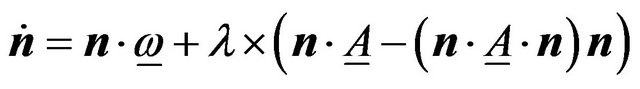
Evolution equation describes the effect of the rheology on directors. This equation considers the directors as if they were pinned on their center of mass and can only spin without translation as described in [7]
 (2)
(2)
The first term on the right hand side of equation accounts for the effect of vorticity tensor,  and the second term is to calculate the effect of strain rate tensor,
  , on the director n
 and
and  are antisymmetric and symmetric parts of the velocity gradient tensor. λ is the tumbling factor defined in [2] which shows the relative importance of the effect of vorticity tensor to the strain rate tensor. Three different regions for λ are normally considered. λ < 1 is associated with the case that the effect of vorticity tensor dominates and tumbling of directors occurs. λ > 1 is the case in which the effect of strain rate tensor is dominant and results in alignment of directors and λ = 1 is the pseudo-affine case. Based on discussions of [8], the value λ = 1 is considered here for thermotropic liquid crystalline polymers. Solving the vector Equation (2) gives the change of the director n with time in three principal directions namely
 and
and . By having the time steps of the simulation,
changes in the director,  and its three components dnx, dny and dnz can be calculated for each cell.
2.3. Franks Elastic Energy
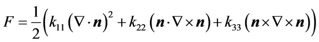
The equation for the curvature distortion energy in liquid crystals is developed by [4] and [9]:
 (3)
(3)
in which k11, k22 and k33 are material constants known as Franks elastic constants for splay, twist and bend respectively and n is director. In simple geometries [3] solved this equation with different values for splay, twist and bend constants. Franks elastic constants are in the order of 10−10 N and the relation between Franks elastic constants and molecular properties of liquid crystals are derived by [10,11].
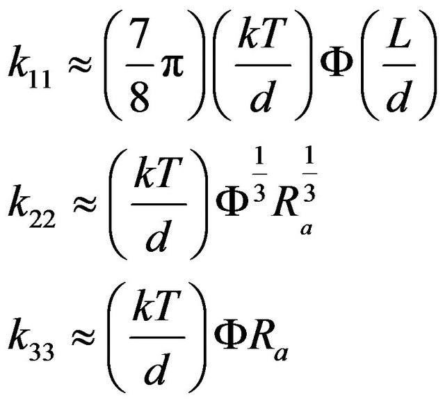 (4)
(4)
In Equation (4), L is the contour length, k is the Boltzmann constant, Ra is the ratio of q (persistence length) to the diameter d of the chain, Ф is the volume fraction which since we are dealing with thermotropic liquid crystalline polymers is considered to be one and T is the temperature. For LCPs, Franks elastic constants are not equal and it is shown by [12] that more features of LCPs can be modeled when larger value of splay constant is considered compared to bend and twist. In small molecule liquid crystals, Franks elastic constants are almost equal.
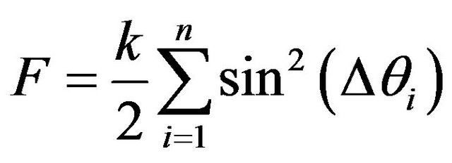
In this study, it is assumed that inside the polymer the average alignment of crystals in each cell can be represented by a director. Moreover, for the sake of simplicity in numerical calculations Franks elastic constants are considered to be equal. In this special case, Equation (3) can be approximated by Equation (5) which can be applied to a meshed geometry [13].
 (5)
(5)
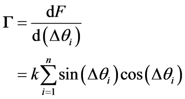
In Equation (5), k = k11 = k22 = k33 and the summation is over all the neighboring cells which have a common surface with the central cell.  is the difference between the angle of the central cell and its i-th neighbor. The torque applied to the central cell can be calculated by taking the derivative of the distortion energy with the angle
 .
.
 (6)
(6)
The torque  , is the result of distortion in the liquid crystals. Since for the two dimensional case the direction of the torque vector is always perpendicular to the plane of flow, it is possible to do the algebraic summation over all the neighbors to find the resulting torque applied to the central cell. In contrary, in three dimensional cases the effect of each neighbor on the central cell should be calculated separately and added like vectors. In three dimensional geometries the effect of each neighbor on the central cell will result in a torque which is normal to the plane that passes through the two directors if they had the same origin. As a result, the total torque applied to the central cell is the vector summation of these individual torques.
After finding the resultant torque applied to the central cell, one can find the rate of change of direction of the director as
 (7)
(7)
In Equation (7),  is the rotational viscosity which based on [14] for thermotropic liquid crystalline polymers (Ф = 1) and can be approximated as
 (8)
(8)
In which  is an empirical constant in the order of 10−4 [15]. For a specific Vectra—a material with typical viscosity of
 , rotational viscosity is about
  Pa·s [3].
2.4. Translation of Directors
Evolution and Franks energy equations assume the director to be fixed in place and can only spin around their center of mass. However, in real flow, directors will be translated with the bulk of material which needs to be accounted for in the numerical simulation. Since in this study different element types and orientation needs to be accounted for, a new method for simulating the translation of directors is developed. The translation of directors is calculated from one element to the neighboring ones based on the direction and velocity of the flow for each element. Figure 1 shows a simple case in which quadriclateral central cell, c, is surrounded by four other cells i = 1 ··· 4.
The method used here assumes that the velocity V transfers bulk of fluid to cell i only if . So for the mesh shown in Figure 1, bulk of fluid is transferred from central cell to the 1st and 2nd neighbor due to acute angle between V and Ai. The important step in this simulation is that the change needed for all the cells should be calculated and added together before applying it to the neighboring cell because of the fact that each cell may receive crystals from more than one neighbor. It is also important to consider the value of the velocity in calculating the transfer of fluid. Here the velocity of fluid in each cell is compared to the distance between cell centers to determine how each cell affects its neighbors. This method can be applied to cells regardless of their number of faces in 2 and 3 dimensions.
2.5. Boundary Conditions
Three types of boundary condition namely planar, homeotropic and tilted can be applied to the directors on the boundaries of the flow in simulating Franks elastic energy. These boundary conditions are shown in Figure 2. These orientations for directors can be achieved experimentally by treating the surface of the wall [16]. In this
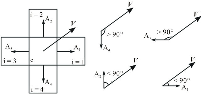
Figure 1. Translation of directors.
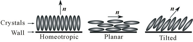
Figure 2. Boundary conditions on directors.
study, planar and homeotropic boundary conditions are applied in different situations. In two dimensions, homeotropic and planar boundary conditions do not need any extra information to be defined.
In three dimensions, planar boundary condition needs one angle,  and tilted boundary condition needs two angles
  and Ф to be defined. Effect of these boundary conditions propagates inside the bulk of fluid and affects the orientation of directors inside.
3. Numerical Method
3.1. Modeling Rheology
As mentioned before, modeling rheology is done using ANSYS® FLUENT® Release 13.0.0. The geometry of the flow is modeled in a 2D channel and meshed with triangular and quadrilateral mesh for comparison. As modeling directionality is of prime interest, the accuracy of the calculations for modeling rheology is of little importance. As a result, first order upwind scheme is used in isothermal solver. The more accurate the rheology modeling, the more accurate one can predict the effect of rheology on the crystals. For modeling the fluid, capillary rheometer data using a LCR 6000 capillary melt rheometer is used for a LCP material in 350˚C temperature. Capillary rheometry data shows close match between the stress-strain curve and power-law model and as a result, power-law model with flow consistency index of k = 1864 Pa·sn and power-law index of n = 0.465 1is considered.
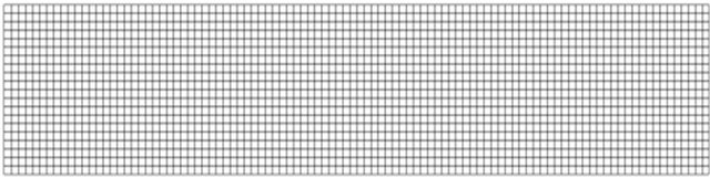
Figure 3 shows the structured and unstructured mesh used for this study.
 (a)
(a)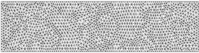 (b)
(b)
Figure 3. (a) Structured and (b) unstructured mesh used for simulations.
3.2. Modeling Directionality
As described above, the directionality simulation used in this study has been implemented with user defined functions (UDFs) in Fluent. UDFs are powerful tools available in ANSYS® FLUENT® to increase the capabilities of ANSYS® FLUENT®. Since all the code written for UDFs are in C++ language, it is possible to utilize all the capabilities of C++ programming and functions for the calculations. There is no readily available tool in ANSYS® FLUENT® to simulate the directionality of fluid in the shear flow; as a result, UDFs are used for this simulation. Here three independent functions are used to show the effect of Franks elastic equation, evolution equation and translation of directors. Vorticity tensor,  and strain rate tensor,
  should be built by extracting the velocity gradients in different directions from the solver. Six user defined memories (UDMs) are needed in 2D to complete the calculation. UDMs are defined to store a variable for each cell in ANSYS® FLUENT®. It is possible to store the components of a director for each cell using UDMs.
4. Results
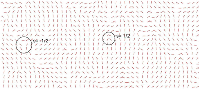
The result of applying the Franks elastic energy function to randomly generated directors is shown in Figure 4. Two of the disclinations existed in the structured mesh are shown with the strength of . The disclinations are less obvious on unstructured mesh because of the random placement of directors in the domain. In this figure, the final minimum elastic energy of the system (Equation (5)) in structured and unstructured cases are calculated to be the same.
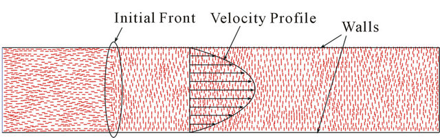
The result of applying the effect of shear to a randomly generated director field on (a) structured and (b) unstructured mesh is shown in Figure 5. As can be seen, the effect of shear penetrated inside the fluid. The flow entering the channel from left has a uniform velocity profile and as it moves through the channel, the boundary layer develops and makes the directors aligned to the direction of flow. In both cases of structured and ustructured meshes, the initial random directors remain undisturbed in the middle of the channel where there is minimum shear.
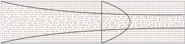
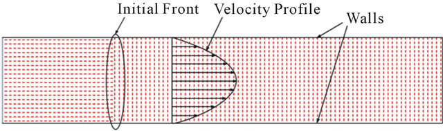
Figures 6 and 7 show how the described method for translating the directors affects the director field. The meshes considered for this calculation are the same meshes used in previous calculations and the initial condition is such that  of the directors are positioned vertically and in the rest of the domain directors are positioned horizontally. The mass flow rate is lowered in this calculation so that all the stages of translation of directors can be visu-
 (a)
(a) (b)
(b)
Figure 4. Effect of Franks elastic energy on directors on (a) structured mesh and (b) unstructured mesh.
 (a)
(a)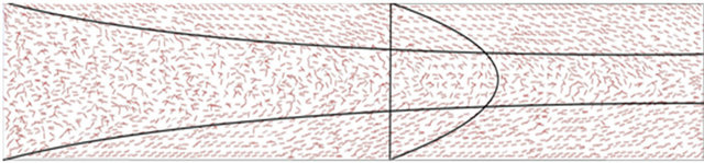 (b)
(b)
Figure 5. Effect of shear on directors in (a) structured mesh and (b) unstructured mesh.
 (a)
(a)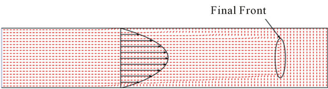 (b)
(b)
Figure 6. Effect of translation of directors with bulk of fluid on directors. (a) Initial condition; (b) Final condition.
 (a)
(a)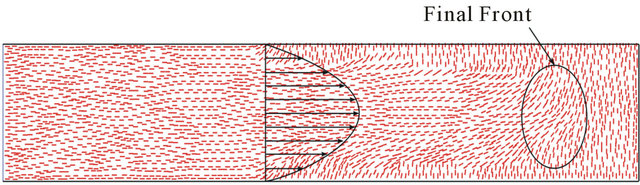 (b)
(b)
Figure 7. Effect of translation of directors with bulk of fluid on unstructured mesh: (a) Initial condition; (b) Final condition.
alized. As can be seen, the lower velocity of fluid in the boundary layer is preventing the flow to transfer the directors to the nearby cells. On the other hand, higher velocity of the bulk of fluid in the center of the channel transfers the directors to the downstream cells completely.
5. Conclusion
A novel method of applying the main components of modeling directionality is developed and effects of each component on the directors is presented on different meshes. It is shown that this method can be applied to different grid types and their combinations which makes it suitable for practical applications with complex geometries. In this study different time constants are considered for different components of flow simulation to visualize their effects on directors.
REFERENCES
- F. M. Leslie, “Some Constitutive Equations for Liquid Crystals,” Archive for Rational Mechanics and Analysis, Vol. 28, No. 4, 1968, pp. 265-283.
- J. Ericksen, “Transversely Isotropic Fluids,” Colloid and Polymer Science, Vol. 173, No. 2, 1960, pp. 117-122.
- G. Goldbeck-Wood, P. Coulter, J. R. Hobdell, M. S. Lavine, K. Yonetake and A. H. Windle, “Modelling of Liquid Crystal Polymers at Different Length Scales,” Molecular Simulation, Vol. 21, No. 2-3, 1998, pp. 143-160.
- F. C. Frank, “I. Liquid crystals. On the Theory of Liquid Crystals,” Discussions of the Faraday Society, Vol. 25, 1958, pp. 19-28.
- Ansys, “FLUENT, Version 13,” Ansys Inc., Canonsburg, 2010.
- A. Ahmadzadegan, A. Saigal and M. A. Zimmerman, “Investigating the Rheology of LCPs through Different Die Geometries,” In: J.-Y. Hwang, S. N. Monteiro, C.-G. Bai, J. Carpenter, M. Cai, D. Firrao and B.-G. Kim, Eds., Characterization of Minerals, Metals, and Materials, John Wiley & Sons, Hoboken, 2012. doi:10.1002/9781118371305.ch41
- A. M. Donald, A. H. Windle and S. Hanna, “Liquid Crystalline Polymers,” Cambridge University Press, Cambridge, 2006. doi:10.1017/CBO9780511616044
- M. S. Lavine and A. H. Windle, “Computational Modelling of Declination Loops under Shear Flow,” Macromolecular Samposia, Vol. 124, No. 1, 1997, pp. 35-47. doi:10.1002/masy.19971240107
- C. W. Oseen, “The Theory of Liquid Crystals,” Transactions of The Faraday Society, Vol. 29, No. 140, 1933, pp. 883-899.
- T. Odijk, “Theory of Lyotropic Polymer Liquid Crystals,” Macromolecules, Vol. 19, No. 9, 1986, pp. 2313-2329.
- R. B. Meyer, A. Cifferi and W. R. Krigbaum, “Polymer Liquid Crystals,” Academic Press, New York, 1982.
- J. Hobdell and A. Windle, “A Numerical Technique for Predicting Microstructure in Liquid Crystalline Polymers,” Liquid Crystal, Vol. 23, No. 2, 1997, pp. 157-173.
- A. H. Windle, H. E. Assender, M. S. Lavine, A. Donald, T. C. B. McLeish, E. L. Thomas, A. H. Windle, et al., “Modelling of Form in Thermotropic Polymers and Discussion,” Philosophical Transactions of the Royal Society of London. Series A: Physical and Engineering Sciences, Vol. 348, No. 1686, 1994, pp. 73-96.
- M. Doi and S. F. Edwards, “The Theory of Polymer Dynamics,” Oxford University Press, Oxford, 1988.
- R. G. Larson, “On the Relative Magnitudes of Viscous, Elastic and Texture Stresses in Liquid Crystalline PBG Solutions,” Rheologica Acta, Vol. 35, No. 2, 1996, pp. 150- 159.
- L. T. Creagh and A. R. Kmetz, “Mechanism of Surface Alignment in Nematic Liquid Crystals,” Molecular Crystals and Liquid Crystals, Vol. 24, No. 1-2, 1973, pp. 59- 68. doi:10.1080/15421407308083389