Natural Resources
Vol.06 No.12(2015), Article ID:61849,13 pages
10.4236/nr.2015.612053
Exploring Emergent Vegetation Time-History at Malheur Lake, Oregon Using Remote Sensing
Zola Yaa Apoakwaa Adjei, Mackayla J. Thyfault, Gustavious Paul Williams
Department of Civil and Environmental Engineering, Brigham Young University, Provo, UT, USA

Copyright © 2015 by authors and Scientific Research Publishing Inc.
This work is licensed under the Creative Commons Attribution International License (CC BY).


Received 27 October 2015; accepted 8 December 2015; published 11 December 2015

ABSTRACT
The extent of emergent vegetation can be a useful indicator of lake health and identify trends and changes over time. However, field data to characterize emergent vegetation may not be available (especially over longer time periods) or may be limited to small, isolated areas. We present a case study using Lands at data to generate indicators that represent emergent vegetation extent in the near-shoreline and tributary delta areas of Malheur Lake, Oregon, USA. Malheur Lake has a large non-native carp population that may significantly affect emergent vegetation and adversely impact reservoir health. This study evaluates long-term trends in emergent vegetation and correlation with common environmental variables other than carp, to determine if emergent vegetation changes can be explained. We selected late June images for this study as vegetation is relatively mature in late June and visible, but has not completely grown-in providing a better indication of vegetation coverage in satellite images. To explore trends in historic emergent vegetation extent, we identified eight regions-of-interest (ROI): three inlet areas, three wet-shore areas (swampy areas), and two dry-shore areas (less swampy areas) around Malheur Lake and computed the Normalized Difference Vegetation Index (NDVI) using 30 years of Lands at images from 1984 to 2013. For each ROI we generated time-series data to quantify the emergent vegetation as determined by the percent of area covered by pixels that had NDVI values greater than 0.2, using cutoff as an indicator of vegetation. For correlation, we produced a corresponding time series of the lake area using the Modified Normalized Difference Water Index (MNDWI) to identify water pixels. We investigated the correlation of vegetation coverage (an indicator of emergent vegetation) with lake area, June precipitation, and average daily maximum temperatures for a period from two months prior to one month after the June collection (April, May, June, and July); all parameters that could affect vegetation growth. We found minimal correlation over time of the vegetative extent in any of the eight ROIs with the selected parameters, indicating that there are other factors which drive emergent vegetation extent in Malheur Lake. This study demonstrates that Landsat data have sufficient spatial and temporal detail to provide insight into ecosystem changes over relatively long periods and offers a method to study historic trends in reservoir health and evaluate potential influences. We expect future work will explore other potential drivers of emergent vegetation extent in Malheur Lake, such as carp populations. Carp were not considered in this study as we did not have access to data that reflect carp numbers over this 30 year period.
Keywords:
Remote Sensing, Emergent Vegetation, Land Sat, NDVI Time Series, MNDWI

1. Introduction
1.1. Study Objectives
This study extends recent work evaluating long-term reservoir and lake water quality trends by using historic Landsat data to create and analyze time series of various water quality indicators [1] - [3] . This study analyzes the time history and changes in near shore-line emergent vegetation at Malheur Lake from 1984 to 2013.
Malheur Lake has a large non-native carp population that affects water quality and emergent vegetation. We do not have data on historic carp population, so this study evaluates whether other environmental drivers could explain trends in emergent vegetation, or if the trends are due to parameters not considered in this study―such as carp. We examined the correlation of emergent vegetation time series with a number of parameters that could influence the extent of emergent vegetation to determine if changes could be attributed to these factors.
1.2. Malheur Lake
Malheur Lake (Figure 1), a terminal lake that has an average area of 35,000 to 45,000 acres (14,000 to 18,000 hectares) with an approximate volume of 85,000 acre-feet (100 million cubic meters) and an elevation of about 4, 000 feet (1200 meters). The average depth is approximately 2 feet with a maximum depth of 5 feet (0.6 to 1.5 meters). The primary inflows are the Donner und Blitzen River, the Silvies River, and Sodhouse Spring with a total watershed of approximately 3000 square miles (~8000 square kilometers). Malheur Lake water flows into Mud Lake during above average water years and is a terminal lake in other years. In extreme flood conditions, Malheur, Mud and Harney Lake become one alkaline lake with no outflow.

Figure 1. A false-color Landsat 7 image of Malheur Lake acquired on July 30, 2013. Malheur Lake is the location of the Malheur Lake National Wildlife Refuge in Harney County, Oregon.
Malheur Lake is located in the Malheur National Wildlife Refuge which was established on August 18, 1908 as the Lake Malheur Bird Reservation, and is located 30 miles south of Burns, Oregon in the southeast corner of the state (Figure 1 upper right inset). While the Refuge’s primary mission is to conserve habitat of the resident 320 species of birds and 58 mammals; fish habitat has become an important aspect of the habitat management program. As part of this program the Refuge has implemented research studies to help understand how fish use the waterways and impact the environment.
In the 1950’s, common carp (Cyprinus carpio) were introduced to Malheur Lake with significant impacts to the ecological systems; in the absence of predators, carp numbers exploded leading to decreased native submerged plant communities and diminished waterfowl use; estimated at 10% - 20% of historic values.
One of the biggest challenges in understanding the impacts carp have had on bird use at the refuge are determining how the carp affect the emergent vegetation in wetlands and ponds―especially trying to determine historic trends. Since carp are bottom feeders, sifting through mud searching for insects and plants, they can significantly impact wetlands [4] . Carp not only uproot emergent vegetation, but feeding can also produce silt plumes in the water column, which makes it difficult for plant photosynthesis and insect production.
The Refuge has begun a number of studies, including this work, to better understand water quality and historic trends and to determine the various system drivers. This study specifically looks at late-June near-shoreline vegetation extent, as an indicator of emergent vegetation, and evaluates water levels, spring temperatures, and June precipitation as potential drivers. Carp populations were not evaluated as we do not have good historic data.
1.3. Remote Sensing
Remote sensing provides useful data that can be used to uniquely study complex environmental issues because of the extent of the coverage in time and space and the minimal cost of data collection. Remote sensing has proven to be an effective method for monitoring single lakes or comparing different lakes over a long time periods [5] . The Landsat Thematic Mapper (TM) sensor is especially useful because of its archival data set that can support long-term historic studies and spatial and spectral characteristics suitable for analyzing reservoir conditions of interest [2] [3] [6] . Although Landsat TM provides a long term archive of spatial data, relatively few studies have reported using this sensor to assess and analyze long term trends. TM spatial resolution is approximately 30 meters (m) and includes eight spectral bands. The size of the Malheur Lake used in this study, is large enough that the 30 m pixel resolution well suited for evaluating reservoir conditions [7] .
Spatial water quality analysis applications are commonly performed using remote sensing approaches―typi- cally looking at chlorophyll distributions as an indicator of algal populations [1] - [3] [8] - [11] . This area is still an active area of research with new methods recently reported such as a sub-seasonal approach based on algal succession to generate time histories of seasonal phytoplankton population changes in reservoirs [1] - [3] . These long-term studies report metrics such as reservoir averages, maximums, and other estimates of chlorophyll-a concentrations over a growing season, information that may not be available historically and data that are not feasible to collect with in-field sampling. As Landsat data are available over a nearly 40 year period, long-term trends in reservoir water quality can be identified and studied [1] - [3] . Hansen et al. [1] - [3] presented case studies that covered a period of 30 years―demonstrating the use of historic remote sensing data to study long-term trends in reservoir water quality. For many reservoirs or lakes, historic field data do not exist and remote sensing is the only method available to generate time histories.
Landsat data are also used to study the extent and type of vegetation coverage. The resolution of datasets from LANDSAT, SPOT, and MODIS satellites provide sufficient spatial resolution for quantification and descriptionsof vegetation coverage and are also appropriate for analyzing land-use/cover changes over time [12] - [14] . Spectral band ratios and combinations are used to calculate various vegetation indices to quantify the extent and type of land cover [15] - [17] . These indices exploit the spectral differences between vegetation and other ground cover types. This is based on the fact that vegetation exhibits strong absorbance in the red regions of the spectra and strong reflectance in the near-infrared part of the spectrum which allows vegetation to be identified [18] - [21] . Singh’s comparison [18] of different indices showed that the most accurate index for detecting change in vegetation is the Normalized Difference Vegetation Index (NDVI).
Although many studies use NDVI to identify fairly dense plant coverage such as grasslands, shrubs or thorny trees in the ecosystem, the reflectance of emergent plants and other aquatic species have been less studied because of the difficulty in understanding results because of issues related to water absorption in the infrared and how this affects mixed pixels (i.e., pixels that include both water and vegetation) [16] [17] . There have been some studies using spectral data, but with different sensors. In Searsville Lake in coastal central California, the reflectance spectra of aquatic vegetation have been studied using a high resolution hand-held spectroradiometer [22] . The size of the lake (approximately 49 acres) makes suitable for analysis using a hand-held spectral camera to capture a few small regions on the lake and extrapolating to the entire reservoir, an approach that is not suitable for large lakessuch as Malheur. Landsat also has deficits, such as a significantly lower spectral resolution than the spectral camera used in the reported study.
There are methods to identify pixels covered with water using Landsat data. A common approach is the Modified Normalized Difference Water Index (MNDWI) which was developed to delineate open water features and enhance their presence in remotely-sensed digital imagery [23] .
For this study we used Landsat-5 TM and Landsat-7 Enhanced Thematic Mapper (ETM) band reflectance values to evaluate the time history of emergent vegetation growth at Malheur Lake. We computed both NDVI and MNDWI spatial extent and change over time for use in this study.
2. Methods
2.1. Study Areas
We selected eight regions-of-interest (ROIs) on the reservoir perimeter as our study areas. We assume that late-June vegetation extent in near-shore areas can be used as an index to emergent vegetation. We selected ROIs representing three different near shore area types. The ROIs used in this study are shown in Figure 2.
ROIs locations and boundaries were selected using an image from a wet year (1984). If a dry year had been used there could be potential error as much of the area in the ROIs would be covered with water in high water years, yielding negative values of NDVI. This means that during dry years a larger percentage of the ROI areas are dry―but this correctly reports vegetation extent. Eight ROIs were chosen: three inlet areas, three wet-shore areas (swampy areas), and two dry-shore areas (less swampy areas). The locations of all 8 ROIs with their labels are shown in Figure 2.
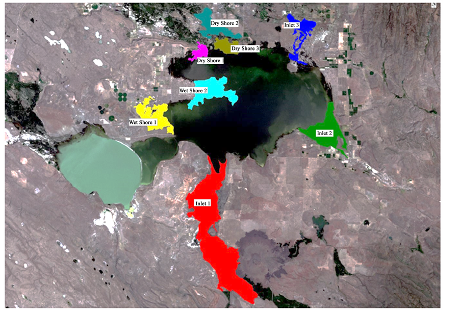
Figure 2. Labelled regions of interest (ROIs) where NDVI data were extracted to examine the trends in emergent vegetation from 1984 to 2013.
To approximately quantify emergent vegetation extents, for each ROI we computed the percent of pixels with an NDVI index from 0.2 to 0.4 in the ROI. The range of 0.2 - 0.4 represents the reflectance associated with emergent plants [24] . This allows us to quantify relative change over time, even though the actual computed area may be less accurate. We use the relative values from year-to-year as indicators of the approximate extent and develop a long-term series that gives insight into the behavior of emergent vegetation over time.
2.2. Satellite Data Calibration and Processing
We obtained both Landsat 5 TM and 7 ETM images as Geotiff files from the USGS Explorer website. We used data from four consecutive months; April, May, June and July. The typical season of emergent vegetation growth at Malheur Lake, based on observations from lake ecologists, is from mid-June to late-June. Data covered the span from 1984 to 2013. The Landsat images which include Malheur Lake are located within path 43 and row 30 of the Landsat satellite orbit.
We calibrated and corrected the Landsat data to remove atmospheric effects. Atmospheric effects are similar to haze that can be seen when looking over large distances. Landsat 7 images acquired after May 2003, such as those used in this study, often exhibit black stripes which are missing pixels in the image due to a scan line correction (SLC) failure on the satellite, and can cause errors in averaging NDVI values if the failed pixels are included in the average. Pixels affected by either SCL failures or clouds cannot be used to estimate vegetation coverage. We excluded these pixels from our calculations.
We used standard routines in ENVI [25] to calibrate and correct the satellite images to remove atmospheric effects and standardize the data. This calibration adjusts the data to represent top of the atmosphere reflectance values in the range from 0 - 1. Calibration requires satellite gains and offsets, solar irradiance, sun elevation, and acquisition time as input. These values are contained in the metadata associated with the Landsat 5 and 7 images. Initial calibration was done using:
 (1)
(1)
where Lλ is radiance in units of W/(m2 * sr * µm) measured by the sensor, d is the earth to sun distance in astronomical units, Sλ is the solar irradiance in unites of W/(m2 * µm), and θ is the sun elevation in degrees. After applying Equation (1) we then corrected the images using a dark subtraction algorithm. This algorithm locates the pixel with least recorded reflection and assumes that amount can be attributed to interferences (or backscatter) from the atmospheric column. That amount is then subtracted from all other pixels, correcting or removing the reflectance caused by atmospheric interference. Since this work was completed, the United States Geological Survey (USGS) has provided calibrated Landsat data as the CDR data set.
2.3. Normalized Difference Vegetation Index Analysis
We used NDVI to compute the extent of vegetation in the selected ROIs over time. NDVI is the most widely used method in mapping vegetation with Landsat data because it produces the best discrimination statistics and provides data for visual interpretations from images [18] [26] . NDVI is calculated as a normalized transform of the near-infrared (NIR) band and red band reflectance ratio and is an index of the absorptive and reflective characteristics of vegetation in the red and near-infrared portions of the electromagnetic spectrum.
The NDVI is computed as:
 (2)
(2)
where NIR (Landsat Band 4) and RED (Landsat Band 3) represents the amount of near-infrared and red light, respectively, reflected by the vegetation and captured by the satellite sensor [27] . The NDVI is based on the principle that chlorophyll absorbs light in the red spectral region (Landsat band 3) and the mesophyll leaf structure scatters light in the near-infrared spectral region (Landsat band 4). We use NDVI to estimate plant cover, and by implication emergent vegetation extent, on the perimeter of Malheur Lake in eight ROIs; for this study it is assumed late-June vegetation cover area can be used as an indicator for emergent vegetation. Late-June vegetation was selected to use as an indicator as by this date vegetation is visible, but not completely grown in, so areal coverage estimates are more accurate.
One issue with NDVI data sets is the problem of mixed pixels [14] [15] . Mixed pixels result when a single pixel encompasses areas of water, land, and vegetation. Traditionally NDVI is used over land, not water, and the NDVI value can be used as an indication of what percent of a pixel is covered with vegetation―though correlations change for different types of plants. However, when a pixel includes vegetation, water, and land, a lower NDVI value results compared to a pixel with the same plant cover percentage with only mixed land and vegetation because: pure water pixels have a negative NDVI value. For this study enough pixels have been used (several thousand in each ROI) we believe that on average the general trends in emergent vegetation are correct, even though the actual ground cover percentage may not be precise. In acknowledgement, the data are not presented as a percent plant cover, but rather as a non-dimensional index to emergent vegetation.
There are other potential documented issues with NDVI values such as the effect of cloud contamination, varying solar zenith angles and surface topography, which can be minimized using a maximum value compositing procedure [6] [14] [28] . The method smooths NDVI time series where the highest NDVI value for the period and area considered is retained. A similar procedure for removing noise in NDVI datasets uses the average of NDVI values in an ROI and yields similar results to the maximum value compositing approach. For this study we calculated the average values of pixels with NDVI values in the range of 0.2 - 0.4. This is essentially a weighted average of the pixels in an ROI, so we did not use the maximum value compositing method.
To analyze long-term emergent vegetation drivers in the eight ROIs, we computed the correlation of the NDVI time series with the time series of various potential drivers of emergent vegetation: lake level, June precipitation, and average maximum temperatures for April, May, June, and July. Similar approaches have been used in other studies which try to identify the drivers of change in emergent vegetation and biomass patterns [12] [29] [30] . These studies all showed a positive correlation of rainfall and temperature time series with NDVI values, especially during the growing seasons.
We computed NDVI values using the NDVI routine in the ENVI software. The output is a single band image with pixel values ranging from −1 to 1, with negative values indicating an absence of vegetation [27] . The intermediate values represent the condition or extent of vegetation in a pixel. A value of approximately 0.6 to 0.9 corresponds to dense vegetation such as temperate and tropical forests or crops at their peak growth stage, sparse vegetation such as shrubs and grasslands or senescing crops result in moderate NDVI values of approximately 0.2 to 0.4 and areas of barren rock, sand, or snow show very low NDVI, for example 0.1 or less [24] . Water typically has a negative NDVI value.
We computed NDVI values for each available April, May, June and July Landsat image from 1984 to 2013. For each ROI, we calculated the pixel statistics in 4 different ranges. We selected these ranges to group the different conditions of vegetation in the sample regions. The ranges were 0.2 - 0.4, 0.4 - 0.6, 0.6 - 0.8 and 0.8 - 1.0. For the pixels in each ROI and in each range, the average, minimum, maximum, kurtosis, and skew values were calculated. Although the Skew and Kurtosis were calculated they were not analyzed, only the average NDVI for the months of April to July from 1984 to 2013 were analyzed [12] . The average in each range provides an index to the plant cover in that ROI and is weighted average that represents a spatial area. As noted above, we did not attempt to compute actual areas, but instead assume that the change in area between images is accurate (even though the actual computed area may not be).
2.4. Modified Normalized Difference Water Index
Landsat images (the same images used to compute NDVI to match in time) were used to determine lake area. We computed the lake area using the Modified Normalized Difference Water Index (MNDWI) to identify pixels that represented water, and then summed the area of each individual water pixel to determine lake area. Malheur Lake area (Lake Area Index) was computed for each late-June Landsat image from 1984 to 2013. The MNDWI index was originally developed to delineate open water features and enhance their presence in remotely-sensed digital imagery. The initial normalized difference water index (NDWI) used a ratio of the near-infrared band (Landsat Band 4) and the visible green (Landsat Band 2) to identify water pixels [31] . The NDWI was modified (called the MNDWI) for greater enhancement of water by using the short wave infrared band (Landsat Band 5) of the Landsat sensor in place of the near-infrared band [23] . The MNDWI is calculated as follows:
 (3)
(3)
where GREEN (Landsat Band 2) is the band in the green region of the spectra and SWIR (Landsat Band 5) is the band in the short-wave infrared region of the Landsat TM sensor. MNDWI represents water features with greater positive values as water has higher absorption in the short-wave infrared region than in the near-infrared region. This approach proved to be a very useful method for estimating reservoir area as shorelines are constantly changing and information on the lake area can be difficult to measure for lakes or reservoirs without monitored outfalls or good bathymetry. Similar to the manner in which NDVI has proven to be a simple and effective method in mapping vegetation, MNDWI has been used in several remote sensing applications to map shores or compute the volume of water in lake ecosystems [32] [33] .
We report the Lake Area Index in units of pixels rather than more standard area units because the actual lake area might be somewhat different because of mixed pixels, but the relative area over time should be accurate. The lake area for a wet year (1984) was delineated and used as the clipping image for all the other years to eliminate other water filled regions such as wetlands or Mud Lake from the calculations (Figure 3).
2.5. Statistical Analysis
We used SAS JMP 11.0 software to perform trend analysis, compute correlations, and generate plots. We validated the normality of the data in the times series (an assumption required for linear correlation computation) by examining the skew and kurtosis values. R-squared values were calculated to determine correlation of the emergent vegetation with the various potential drivers.
3. Results and Discussion
3.1. Data Distributions
We evaluated the distribution of NDVI values in each of the selected ROIs to evaluate whether the ROIs groups we assigned (Inlet, Dry Shore, and Wet Shore) represented similar conditions. If the ROIs contain data that provides a similar distribution, we have more confidence that the selected areas are grouped correctly and represent the three categories assigned for this study. NDVI histograms from the 8 ROI regions are shown in Figure 4. In these histograms, only the data above 0.2 are shown. Data values below 0.2 represent either bare earth or water.
The histograms in Figure 4 show that inlet ROI areas have similar data distributions. This is true even though Inlet 3 is significantly larger than the other two inlets, though Inlet 1 does exhibit more established vegetation (values closer to 0.4) than the other two inlet ROIs. The two Dry Shore ROIs present data distributions similar to
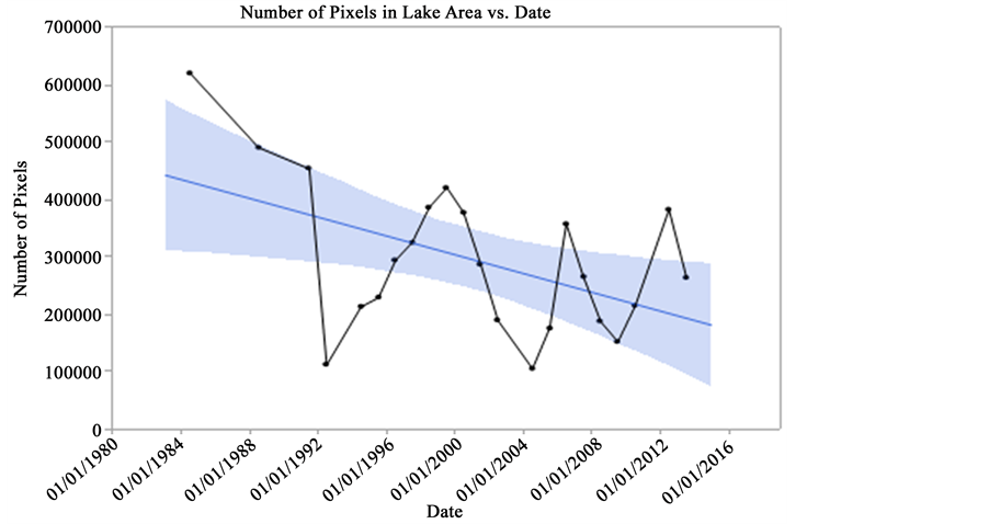
Figure 3. Lake area in late June from 1987-2013 which shows a long-term decreasing trend over the period. Lake area is represented by the number of pixels classified as water in the lake area.
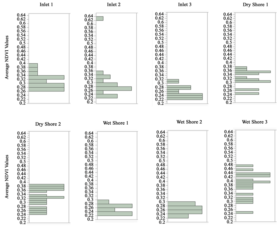
Figure 4. Distribution of NDVI values above 0.2 (inidicative of vegetation) for the 8 ROIs selected for this study.
each other. The Dry Shore ROIs have more data in the dry dirt range than the Inlet ROIs. The first two Wet Shore ROIs have distributions similar to each other with relatively low NDVI values indicating lighter green vegetation more indicative of emergent plants. Wet Shore 3 does not have data in the lower NDVI range (0.2 - 0.3) and has a significant amount of data above 0.4 indicating more established vegetation, probably dark rushes and cattails that extend well above the water. It does appear different than the other two wet shore ROIs.
3.2. NDVI Times Series Trends
In this section, we present representative time series showing trends of emergent vegetation growth on Malheur Lake at 3 ROIs. We selected Inlet 1, Wet Shore 1 and Dry Shore 1 as the ROIs to present in this paper. The results for the other ROIs are similar, but not included here.
Figure 5 presents the average NDVI values for the pixels in the range from 0.2 to 0.4, which is an indicator for emergent plant spatial extent. As noted, late-June conditions were selected as the best time to use remote sensing data to compute an indicator for emergent vegetation. Some years have missing data because of missing images or images that were not useable because of cloud cover or other issues. We were able to use 22 late-June images over the 30 year time period.
Inlet 1 and Dry Shore 1 had similar time-series with the minimum average NDVI value of 0.25 occurring in 1992. The Wet Shore 1 minimum occurred in 1999 with a value of 0.22. The minimum values in the inlet and dry shore areas, were affected strongly by lake levels, with the minimum in 1992, the year of the lowest lake level.
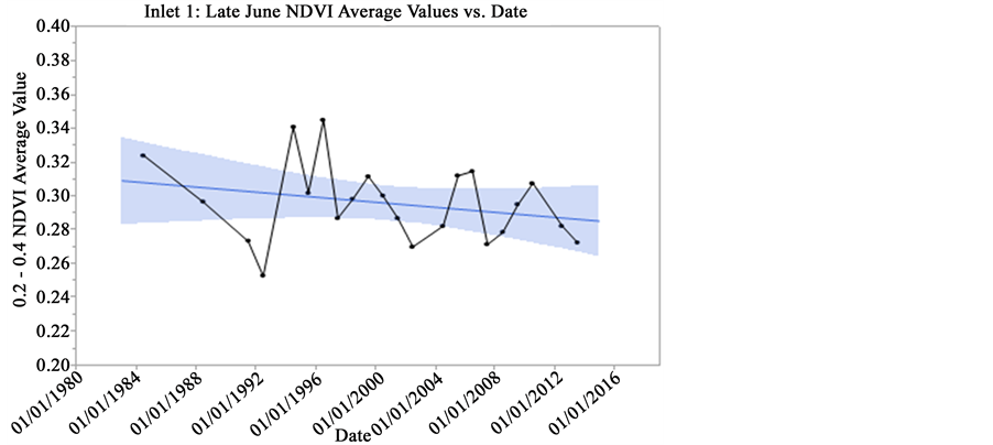
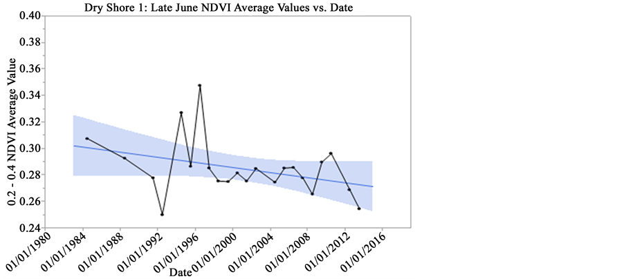
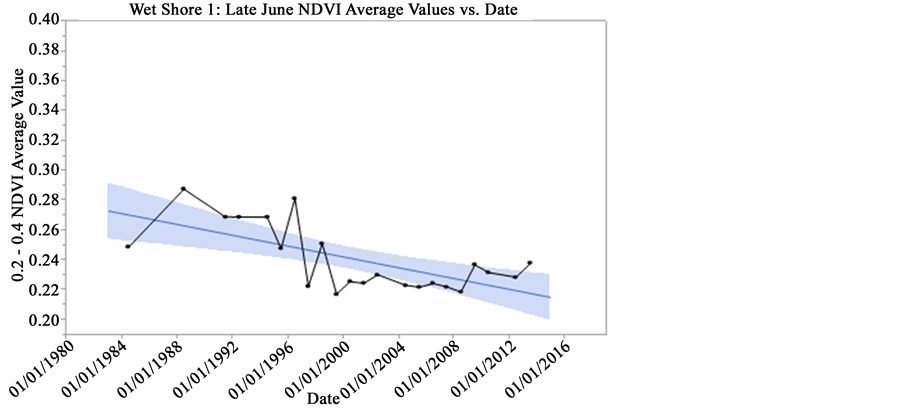
Figure 5. Long term estimated average of NDVI values (0.2 - 0.4 range) in Inlet 1 (top), Dry Shore I (middle), and Wet Shore 1 (bottom) ROIs for late June from 1984 to 2013.
All three ROIs show a declining trend in emergent areal extent over the study period. Values for Wet Shore 1 were comparably lower than the other two sites due to the presence of water which may have influenced with the NDVI values computed for this ROI, though should provide accurate trend estimates for this ROI, as the effect would be similar in each year. The lake level was at a maximum in 1984 (Table 1), which did not necessarily correspond to high NDVI values. Without ground truth data, the actual impact of mixed water pixels on the data cannot be determined, but as noted earlier, the trends should be representative, while the actual values may not be as accurate.
Precipitation (Table 1) shows a slightly increasing trend throughout the study, with significant variability. In 1992, the average daily precipitation was relatively low although not the lowest value in the measurements. June precipitation does not correlate well with lake levels as runoff and lake levels are more dependent on precipitation earlier in the year.
3.3. Correlation of NDVI with Climatic Conditions
This section presents correlations of the vegetation index with other times series which represent climate parameters. Data for temperature and precipitation were obtained from the Oregon Climate Service [34] and as explained, we computed the Lake Area index. We computed R-squared values to quantify the correlation between each of the time series and the NDVI index for emergent vegetation, these values are reported in Table 1. The R-squared values presented Table 1 demonstrate that there is no correlation between any of these times series and the emergent vegetation index.
We plotted the data as shown in Figure 6 to show correlation of emergent vegetation to June temperature (top panel), Lake Area (middle panel), and June Precipitation (bottom panel). We also plotted data for the other variables in Table 1 but they are not shown here. 1992 represented a temperature peak, which does not correlate with an emergent vegetation peak (the other temperature plots were similar). We expected that high temperatures in April would result in greater growth, and a larger emergent vegetation index and conversely, for colder springs the index would be lower. However, even with relatively high temperatures in April of 1992, NDVI values at Inlet 1 were low compared to other years.
The R-squared values for the correlations of April, May June and July average daily maximum temperatures have very weak (to no) correlation. May maximum temperatures have the highest R-squared value, which would be expected as May temperatures could be well reflected in June growth, however, while it is the highest value, it only has a value of 0.0131, which indicates no correlation. These data show that our hypothesis that daily maximum temperature in April, May, June, or July would be a driver for emergent growth, as measured by NDVI, does not hold.
Figure 6 shows (along with Table 1) that the other two variables studied, June daily average precipitation and lake area measurements are not well correlated with emergent vegetation index values either. Lake area exhibits the highest R-squared value of 0.0774, which is the best correlation of all the variables, but is so low as to indicate no correlation.

Table 1. Correlation (R2) of selected parameters with average late-June NDVI values for each ROI.
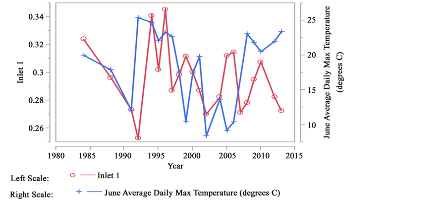
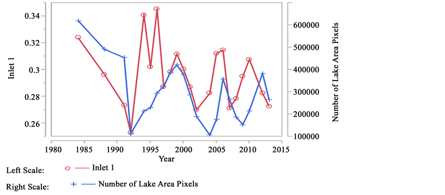
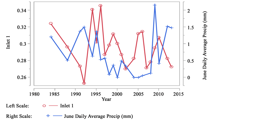
Figure 6. Comparison between NDVI index at Inlet 1 and Malheur Lake data (1984-2013) for June temperature (top), lake area (middle), and June precipitation (bottom).
These results suggest that variation in emergent vegetation cover on the perimeter of the lake, has almost no correlation with any of the parameters evaluated in this study.
4. Conclusions
There are not any strong patterns or trends in the emergent vegetation time series data. We do observe a slight trend represented as a small steady decline year after year in the emergent vegetation index in each of the selected ROIs (Figure 5). This implies that emergent vegetation growth on the perimeter of the Malheur Lake is getting smaller. We analyzed the correlation of emergent vegetation with lake size, June precipitation, and April, May, and June temperature maximum daily temperatures. These data exhibited no correlation with emergent vegetation, indicating that these variables do not drive emergent vegetation conditions.
These results indicate that there are other drivers for emergent vegetation on the perimeter of Malheur Lake. Without additional studies, it is difficult to determine the most important processes and unfortunately, data on carp populations, which are assumed to be a primary driver, do not exist. Additional field studies should also be done to determine if the correct ROIs were selected and if late June is the most appropriate month to use for estimating emergent vegetative extent at Malheur Lake.
The methods developed in this study could be used for on-going reservoir management as Landsat collects data every 16 days and processing, once the method is implemented, is minimal. New remote sensing information could be combined with additional field measurements to explore other correlations and determine the influence of other drivers for the extent of emergent vegetation―such as carp population levels.
Cite this paper
Zola Yaa ApoakwaaAdjei,Mackayla J.Thyfault,Gustavious PaulWilliams, (2015) Exploring Emergent Vegetation Time-History at Malheur Lake, Oregon Using Remote Sensing. Natural Resources,06,553-565. doi: 10.4236/nr.2015.612053
References
- 1. Hansen, C., Swain, N., Munson, K., Adjei, Z., Williams, G.P. and Miller, W. (2013) Development of Sub-Seasonal Remote Sensing Chlorophyll—A Detection Models. American Journal of Plant Sciences, 4, 21-26.
http://dx.doi.org/10.4236/ajps.2013.412A2003 - 2. Hansen, C.H., Williams, G.P. and Adjei, Z. (2015) Long-Term Application of Remote Sensing Chlorophyll Detection Models: Jordanelle Reservoir Case Study. Natural Resources, 6, 123.
http://dx.doi.org/10.4236/nr.2015.62011 - 3. Hansen, C.H., Williams, G.P., Adjei, Z., Barlow, A., Nelson, E.J. and Woodruff Miller, A. (2015) Reservoir Water Quality Monitoring Using Remote Sensing with Seasonal Models: Case Study of Five Central-Utah Reservoirs. Lake and Reservoir Management, 31, 225-240.
http://dx.doi.org/10.1080/10402381.2015.1065937 - 4. Roberts, J., Chick, A., Oswald, L. and Thompson, P. (1995) Effect of Carp, Cyprinus carpio L., on Exotic Benthivorous Fish, on Aquatic Plants and Water Quality in Experimental Ponds. Marine and Freshwater Research, 46, 1171- 1180.
http://dx.doi.org/10.1071/MF9951171 - 5. Dekker, A.G. (1993) Detection of Optical Water Quality Parameters for Eutrophic Waters by High Resolution Remote Sensing. Ph.D. Thesis, Earth and Life Sciences, Amsterdam, The Netherlands. Proefschrift Vrije Universiteit (Free University).
- 6. Fuller, D.O. (1998) Trends in NDVI Time Series and Their Relation to Rangeland and Crop Production in Senegal, 1987-1993. International Journal of Remote Sensing, 19, 2013-2018.
http://dx.doi.org/10.1080/014311698215135 - 7. Sawaya, K.E., Olmanson, L.G., Heinert, N.J., Brezonik, P.L. and Bauer, M.E. (2003) Extending Satellite Remote Sensing to Local Scales: Land and Water Resource Monitoring Using High-Resolution Imagery. Remote Sensing of Environment, 88, 144-156.
http://dx.doi.org/10.1016/j.rse.2003.04.006 - 8. Hansen, C., Williams, G.P., Miller, W. and Adjei, Z. (2014) Development of Sub-Seasonal Remote Sensing Chlorophyll—A Detection Models. Utah Conference on Undergraduate Research, Provo, Utah.
- 9. Han, L. and Rundquist, D.C. (1997) Comparison of NIR/RED Ratio and First Derivative of Reflectance in Estimating Algal-Chlorophyll Concentration: A Case Study in a Turbid Reservoir. Remote Sensing of Environment, 62, 253-261.
http://dx.doi.org/10.1016/S0034-4257(97)00106-5 - 10. Mishra, S. and Mishra, D.R. (2012) Normalized Difference Chlorophyll Index: A Novel Model for Remote Estimation of Chlorophyll—A Concentration in Turbid Productive Waters. Remote Sensing of Environment, 117, 394-406.
http://dx.doi.org/10.1016/j.rse.2011.10.016 - 11. Kutser, T., Metsamaa, L., Strombeck, N. and Vahtmae, E. (2006) Monitoring Cyanobacterial Blooms by Satellite Remote Sensing. Estuarine, Coastal and Shelf Science, 67, 303-312.
http://dx.doi.org/10.1016/j.ecss.2005.11.024 - 12. Anyamba, A. and Tucker, C.J. (2005) Analysis of Sahelian Vegetation Dynamics Using NOAA-AVHRR NDVI Data from 1981-2003. Journal of Arid Environments, 63, 596-614.
http://dx.doi.org/10.1016/j.jaridenv.2005.03.007 - 13. Chen, J., Jonsson, P., Tamura, M., Gu, Z., Matsushita, B. and Eklundh, L. (2004) A Simple Method for Constructing a High-Quality NDVI Time-Series Data Set Based on the Savitzky-Golay Filter. Remote Sensing of Environment, 91, 332-344.
http://dx.doi.org/10.1016/j.rse.2004.03.014 - 14. Pettorelli, N., Vik, J.O., Mysterud, A., Gaillard, J.-M., Tucker, C.J. and Stenseth, N.C. (2005) Using the Satellite-Derived NDVI to Assess Ecological Responses to Environmental Change. Trends in Ecology and Evolution, 20, 503-510.
http://dx.doi.org/10.1016/j.tree.2005.05.011 - 15. Justice, C.O., Townsend, J.R.G., Holben, B.N. and Tucker, C.J. (1985) Analysis of the Phenology of Global Vegetation Using Meteorological Satellite Data. International Journal of Remote Sensing, 6, 1271-1318.
http://dx.doi.org/10.1080/01431168508948281 - 16. Ackleson, S.G. and Klemas, V. (1987) Remote Sensing of Submerged Acquatic Vegetation in Lower Chesapeake Bay: A Comparison of Landsat MSS to TM Imagery. Remote Sensing of Environment, 22, 235-248.
http://dx.doi.org/10.1016/0034-4257(87)90060-5 - 17. Dervieux, A. and Tamisier, A. (1987) Submerged Macrophyte Beds of Camargue Wetlands: Estimation of Their Distribution and Size by the Interpretation of Air Photos. ACTA Oecologica—International Journal of Ecology, 8, 371-385.
- 18. Singh, A. (1989) Digital Change Detection Techniques Using Remotely-Sensed Data. International Journal of Remote Sensing, 10, 989-1003.
http://dx.doi.org/10.1080/01431168908903939 - 19. Tarpley, J., Schneider, S. and Money, R.L. (1984) Global Vegetation Indices from the NOAA-7 Meteorological Satellite. Journal of Climate and Applied Meteorology, 23, 491-494.
http://dx.doi.org/10.1175/1520-0450(1984)023<0491:GVIFTN>2.0.CO;2 - 20. Townshend, J.R., Goff, T.E. and Tucker, C.J. (1985) Multitemporal Dimensionality of Images of Normalized Difference Vegetation Index at Continental Scales. IEEE Transactions on Geoscience and Remote Sensing, GE-23, 888-895.
http://dx.doi.org/10.1109/TGRS.1985.289474 - 21. Middleton, E. and Anuta, M. (1984) Evaluation of the Normalized Difference Vegetation Index with Thematic Mapper Data. 10th International Symposium on Machine Processing of Remotely Sensed Data with Special Emphasis on Thematic Mapper Data and Geographic Information Systems, Purdue University, Laboratory for Applications of Remote Sensing, West Lafayette, 12-14 June 1984, 92.
- 22. Penuelas, J., Gamon, J.A., Griffin, K.L. and Field, C.B. (1993) Assessing Community Type, Plant Biomass, Pigment Composition, and Photosynthetic Efficiency of Aquatic Vegetation from Spectral Reflectance. Remote Sensing of Environment, 46, 110-118.
http://dx.doi.org/10.1016/0034-4257(93)90088-F - 23. Xu, H. (2006) Modification of Normalised Difference Water Index (NDWI) to Enhance Open Water Features in Remotely Sensed Imagery. International Journal of Remote Sensing, 27, 3025-3033.
http://dx.doi.org/10.1080/01431160600589179 - 24. USGS (2015) USGS: Remote Sensing Phenology. US Geological Survey.
- 25. Exelis (2015) Exelis Learn: Tutorials. Exelis Visual Information Solutions.
- 26. Lyon, J.G., Yuan, D., Lunetta, S.R. and Chris, E.D. (1998) A Change Detection Experiment Using Vegetation Indices. Photogrammetric Engineering & Remote Sensing, 64, 143-150.
- 27. Myneni, R.B. and Hall, F.G. (1995) The Interpretation of Spectral Vegetation Indexes. IEEE Transactions on Geoscience and Remote Sensing, 33, 481-486.
http://dx.doi.org/10.1109/36.377948 - 28. Holben, B.N. (1986) Characteristics of Maximum-Value Composite Images from Temporal AVHRR Data. International Journal of Remote Sensing, 7, 1417-1434.
http://dx.doi.org/10.1080/01431168608948945 - 29. Wang, J., Rich, P.M. and Price, K.P. (2003) Temporal Responses of NDVI to Precipitation and Temperature in the Central Great Plains, USA. International Journal of Remote Sensing, 24, 2345-2364.
http://dx.doi.org/10.1080/01431160210154812 - 30. Yu, F., Price, K.P., Ellis, J. and Shi, P. (2003) Response of Seasonal Vegetation Development to Climatic Variations in Eastern Central Asia. Remote Sensing of Environment, 87, 42-54.
http://dx.doi.org/10.1016/S0034-4257(03)00144-5 - 31. McFeeters, S.K. (1996) The Use of the Normalized Difference Water Index (NDWI) in the Delineation of Open Water Features. International Journal of Remote Sensing, 17, 1425-1432.
http://dx.doi.org/10.1080/01431169608948714 - 32. Lu, S., Ouyang, N., Wu, B., Wei, Y. and Tesemma, Z. (2013) Lake Water Volume Calculation with Time Series Remote-Sensing Images. International Journal of Remote Sensing, 34, 7962-7973.
http://dx.doi.org/10.1080/01431161.2013.827814 - 33. Ouma, Y.O. and Tateishi, R. (2006) A Water Index for Rapid Mapping of Shoreline Changes of Five East African Rift Valley Lakes: An Emperical Analysis Using Landsat TM and ETM+ Data. International Journal of Remote Sensing, 27, 3153-3181.
http://dx.doi.org/10.1080/01431160500309934 - 34. OCS (2015) Oregon Climate Data. Oregon Climate Service.