Natural Resources
Vol.4 No.4(2013), Article ID:35150,12 pages DOI:10.4236/nr.2013.44037
A Spatial Analysis of Irrigation Technology
![]()
Department of Agricultural and Applied Economics, Texas Tech University, Lubbock, USA.
Email: andrew.p.wright@ttu.edu
Copyright © 2013 Andrew Wright et al. This is an open access article distributed under the Creative Commons Attribution License, which permits unrestricted use, distribution, and reproduction in any medium, provided the original work is properly cited.
Received March 21st, 2013; revised June 18th, 2013; accepted July 3rd, 2013
Keywords: Technology; Adoption; Water; Irrigation; Natural Resources
ABSTRACT
The nature of spatial spillovers in the adoption of irrigation technology is examined in this paper. Adopting a new technology is a decision that is based on economic and individual-specific factors. One of these individual factors might be communication with other users. It makes sense to expect that contact between users and non-users would follow a spatial pattern, and if knowledge spillovers are important to the adoption decision then resource managers need to be aware of their existence. Using counties in the Texas High Plains as the study area, the adoption of center pivot technology is examined using both Ordinary Least Squares and spatial regression models to determine if knowledge spillovers exist. Ultimately, no evidence was found that adoption practices in a county affects its neighbors; however, geographic location does matter to who adopts and when.
1. Introduction
In the production of a good, the value of a per unit input, and by extension how much of it is used at any given time, is determined in part by the technology related to the input’s use. Ceteris paribus, technological progress decreases the costs faced by firms and increases how much of the input is used in the production process. When the input in question is a stock resource, technological advancement implies that the resource will be depleted at a faster rate.1 It is, therefore, important for anyone whose responsibilities include resource management to understand the process by which technology is adopted by potential users and spreads through a population.
Technology adoption is important to resource management for any number of reasons. The introduction of a more efficient technology changes the incentives faced by producers; thus, any policies that aim at the resource’s conservation may no longer achieve the desired behavior. Consequently, it is important for resource managers to understand which individuals are most likely to adopt the new technology and how the technology will spread over time in order to adjust rules regarding resource use accordingly. On the other hand, policy makers might view more efficient technology as a means to encourage conservation. In this case, understanding the diffusion process will make it easier to identify those individuals or regions that will have the most influence on how quickly the technology spreads.
A real world example of the importance of technology diffusion to resource management is the advancement of irrigation technology in arid regions such as the Texas High Plains. Agricultural production in this region of Texas is a part of the foundation of the region’s economy, and part of the reason for this is the availability of groundwater from the Ogallala Aquifer for irrigation. Over time, producers have found more efficient means of extracting water from the aquifer. Early farms used furrow irrigation to water crops. Sprinklers began replacing furrow irrigation in the mid-20th century; early sprinklers were high pressure systems that required a large amount of energy to operate. In the late 1980s, low energy precision application (LEPA) technology was introduced, and is the primary irrigation technology used today.
As irrigation technology has become more efficient at extracting water from the aquifer, it has become economically viable to irrigate more acres (or irrigate the same acres more intensely). This extraction rate increase has led to concerns about the long-term viability of the aquifer as a resource for irrigation water and the development of plans and policies to curb extraction from the aquifer. In the midst of these concerns, a new irrigation technology has begun to gain prominence, sub-surface drip, which supplies water directly to the root zone of the plant as opposed to sprinklers that deliver water above the surface which is absorbed by the plant through the soil. As such, it is more efficient in its application of water and generally reduces the variable cost of irrigating. Producers, therefore, have an opportunity to increase the amount of water they can take from the aquifer where available, and as drip becomes more prevalent, decision makers concerned about conservation must consider how the spread of this new technology will change water use patterns.
The spread of a technology involves both adoption and diffusion. Adoption occurs when an individual chooses to accept and use the new technology. The decision to adopt can be thought of as an economic choice, where individuals seek to maximize utility or profits [1-4]. Individuals adopt a new innovation if it increases their net revenue from production. This idea has been expanded to acknowledge that individuals are heterogeneous in terms of their preferences as well as the physical and economic factors they must consider when choosing to adopt a new technology [1,2,5].
Diffusion can be thought of as the path that adoption takes through a population over time. Theoretically, the diffusion of technology from one person to another has been closely linked to interactions between individuals [6-11]. As users and nonusers interact, the users of a new technology communicate information about its benefits and its use. Nonusers take this information and use it to decide whether to adopt or not; thus diffusion can be thought of as a process of communication and imitation.
This transfer of knowledge through communication constitutes an information externality associated with the adoption of the new technology. When innovators and early adopters adopt new technology, they take on the costs associated with the risk of using the new technology. Other potential users benefit from the experience of early adopters through person to person transfer of the knowledge gained, and are able to adopt the new technology without the risk involved with early adoption. If the transfer of knowledge is informing adoption decisions, and consequently the diffusion of a technology, then it is necessary to understand the strength of this spillover relative to other factors.
This study examines the presence of information spillovers in the adoption of center pivot systems on the Texas High Plains. Center pivot technology is examined because, as opposed to drip systems, it has reached the end of its diffusion cycle, and there is more reliable data regarding its use. If the adoption of drip technology is determined by similar factors as center pivot systems, then the results of this study can be used as a benchmark for later studies involving drip adoption.
In the study, the number of center pivot systems in each county that is a part of the High Plains Underground Water Conservation District No. 1 (HPWD) is related to the physical qualities of the county such as the saturated thickness of the Ogallala Aquifer at different points in time and the county’s geographic location. These physical characteristics are of particular interest, as it is likely that the area of the aquifer a county overlies will determine how many irrigation systems exist and how quickly this number grows. Furthermore, if there are counties that adopt first then it would be interesting to examine how much influence these counties have on the adoption level of their neighbors, or whether or not information spillovers exists in the adoption process. To this end, spatial econometric models are employed to account for any spatial dependence present in the number of center pivots in each county.
2. Elements of the Adoption/Diffusion Process
The choice to adopt new technology can be thought of as an economic decision where individuals switch to a new innovation because it increases their net revenue from the production of a good. Thus, the decision to adopt will be driven in part by the costs associated with the new technology. References [8] and [10] separate the cost of adopting new innovations into “hardware” costs and “software” costs.
Hardware costs relate to the actual purchase of the technology and its maintenance, and technologies such as irrigation systems that exhibit large hardware costs often rely on a loan to fund the purchase. Thus, access to credit may help these innovations to spread [3,12,13]. Software costs relate to the cost of learning to use a technology, and the ability to learn is related to the concepts of human capital and education. Firms with high amounts of human capital are able to take advantage of their employees’ capabilities and adopt earlier [3,4,13]. Individuals who are better educated can adopt earlier because they face a lower software cost, and due to their greater wealth are better able to afford the hardware costs [14]. Software costs can be reduced through personal experience and communication with existing users, so complicated technologies tend to spread from more skilled users to less skilled users as the stock of knowledge related to the technology increases [8].
Aside from the cost of a new technology, the decision to adopt may be influenced by a number of physical factors as well. While some physical factors, such as firm size, will affect technology adoption in general, these factors are especially important to agriculture due to the relation of agricultural production to physical qualities of the land itself.
Previous studies have found a relationship between the size of a firm and the ability to adopt new technology [15-17]. These authors argue that larger firms are better able to absorb the costs related to adopting a new innovation; thus, there is a lower limit to the size of a firm that can adopt an innovation, and the critical size increases along with the amount of fixed costs involved with the decision. Technology then diffuses from large firms to small firms.
In studies related to irrigation adoption, the effects of land quality, well depth, and water price on adoption have been studied in a variety of frameworks. Land quality, and related factors such as soil type, as well as well depth will determine whether traditional (furrow) irrigation systems or modern (sprinkler or drip) irrigation systems are used [1]. Specifically, the authors show that modern technology is more likely to be adopted on lower quality land, or in areas with deeper wells. Similarly, [18] examines irrigation technology adoption in an exhaustible resource framework and finds that individuals will not adopt modern technology on their highest quality land, but do adopt modern technology as water price increases. Another study of irrigation adoption by [5] confirms the relation between water price and the adoption of modern technology, in this case drip. The authors also find that the adoption of center pivot technology is less sensitive to land quality than that of drip due to the dependence of drip irrigation on field slope [5].
The decision to adopt a new technology is ultimately an individual decision based in part on both economic and physical factors. The difficulty, then, of modeling the adoption process is in collecting individual level data for analysis. The amount of information that must be collected is large, and the time to do so normally intensive. By studying adoption at the aggregate level, as this study proposes to do, the data collection process is much less effort intensive, but many of the micro level variables that affect the adoption decision must be dropped from the study; however, other important features, such as the existence of knowledge spillovers between regions can be explored. Identifying and measuring spillovers requires the use of econometric methods that model spatial dependence between observations. The next section explains how and why these spatial relationships exist and how they might affect a county level analysis.
3. Spatial Relationships and Irrigation Adoption
Spatial location and technology adoption can be linked through the physical location of users and through the geographic relationship between current users and potential adopters. The relationship between physical location and the decision to adopt a new irrigation technology has been explained in detail in the previous section. To summarize, physical characteristics related to an individual’s land will determine where adoption is economically viable. When neighboring counties share similar characteristics, for instance if the saturated thickness of an underlying aquifer is similar, it is reasonable to assume that they will share aggregate irrigation levels as well.
How the geographic relationship between current users and potential adopters affects technology adoption and diffusion is less clear, but not difficult to explain. Early concepts of the diffusion process, [7] for example, modeled the diffusion process as similar to a disease epidemic where the vector is contact between current and potential adopters [10]. As potential adopters come into contact with current users, they are “infected” with the new technology and become users themselves. While these early models did not account for proximity between current and potential users, it should be clear that the probability of contact becomes more likely when the two groups are close to one another. Thus, a technology should diffuse from current users to the individuals closest to them if spatial spillovers are present.
From the above explanation, spatial relationships are clearly important to consider when studying the adoption and diffusion of irrigation technology; furthermore, multiple empirical studies of technology diffusion provide evidence of spatial effects in the diffusion process [19- 21]. With this in mind, the growth of center pivot technologies in the HPWD area is analyzed using a set of spatial regression models. The next section describes the data and variables used in the estimation these models, and the structure of the models themselves.
4. Data and Methods
4.1. Variables and Sources
This study assumes that adoption of irrigation technology will depend on a set of county specific physical factors faced by producers. Irrigation technology adoption is measured using center pivot counts for each county in the HPWD. Information on the number of center pivots systems was provided by the staff of the HPWD [22,23]. The water district collects this information on a semiannual basis only, thus this information was collected for the years 1986, 1990, 1993, 1995, 2005, and 2008, and seven cross sections were developed.
Two measures of saturated thickness are used as independent variables. The first of these is the saturated thickness of the aquifer in the current period. Saturated thickness is closely related to the cost of irrigation, which has been shown to affect the adoption choice [5,18]. It is expected that as the saturated thickness of the aquifer decreases, and the price of pumping water increases, that producers will switch to a more efficient irrigation system. The second variable is the change in saturated thickness over time, and is included to account for the fact that producers might take past experience into account along with current conditions when making the choice to adopt a new technology. In other words, in counties where the reduction in saturated thickness over time is larger, producers might choose to adopt more efficient irrigation technology to extend the life of the aquifer.
Saturated thickness information was collected primarily from the Texas Tech Center for Geospatial Technology (TTUCGT) [24]. The staff at the TTUCGT has developed county average measures of the characteristics of the Ogallala aquifer, such as water storage and saturated thickness. The TTUCGT spans the years 1990-2008. For years prior to 1990, saturated thickness was estimated using the average change in well depth for each county, reported annually in the HPWD newsletter. This calculation started with the 1990 saturated thickness in county i as the baseline, and saturated thickness in the previous year, STt−1, was related to the current year saturated thickness, STt, and change in well depth reported in year t, wt, so that STt−1 = STt − wt.
Other physical characteristics considered in this study are the distance between a county and an experiment station, the amount of irrigated production in a county, and the aridity level in a county. The distance from an experiment station is considered important to the adoption choice because of the role experiment stations play in introducing new technology. These stations act as the central source for information referred to in [6-8], and [10] that introduces the innovation to a population through demonstrations of the new technology. Attending these demonstrations requires that producers travel to the stations, and it is assumed that this will be easier for producers who are closer to a station. There are two experiment stations in the HPWD, so the distance from county to station was calculated as the average distance from the county seat to an experiment station.
The level of irrigated production in a county signifies how willing producers might be to pursuing new irrigation technology. In counties where the amount of irrigated production is high, producers should be more interested in learning about and adopting more efficient irrigation systems. To measure the level of irrigated agriculture practiced in each county, acreage amounts for corn, cotton, sorghum, and wheat where retrieved from the National Agricultural Statistics Service (NASS) quick stats data base [25]. The number of irrigated acres was divided by total acreage to calculate the percent of agriculture that depended on irrigation.
The aridity level in a county indicates how important irrigation is to agricultural production. Producers in counties that are hotter and dryer will rely more on irrigation to supplement natural precipitation, and should be more likely to switch to more efficient irrigation technology when it becomes available. To measure aridity, the Lang Index [26] was calculated for each county in each year. This index is calculated as P/T where P is the annual precipitation in centimeters and T is the average annual temperature in C˚. Temperature and precipitation data was retrieved from the Western Regional Climate Center website [27].
Once the data is collected, it is sorted into seven cross sections, one for each year that the number of center pivots in the HPWD was counted. Each cross section had thirteen observations. There are fifteen counties in the study area; however, only small parts of Armstrong and Potter Counties are actually a part of the HPWD, and these counties practice low levels of crop agriculture. For this reason it is assumed that these counties would have little influence on center pivot adoption in neighboring counties, and would not be influenced by interactions with other counties in the study area. There is some obvious concern about the small number of observations in a given year and the effect on degrees of freedom; however, there is no easy way around this limitation. The accounting procedure for center pivot numbers is only semi-annual in the HPWD which limits the number of years with data available and prevents the use of panel estimation methods; furthermore, expanding the study area to include other water district introduces new concerns such as the effect of differing organizational structures, accounting practices, and data collection procedures.
Additional information collected for this study includes the market average prices reported by NASS and the interest rate for the 3-month T-bill [28]. Crop prices and interest rates may influence the adoption decision; however, while these variables may show variation over time, they do not change from county to county. As the data related to adoption is organized into cross sections, any effect that these variables might have on adoption would simply reduce to a fixed effect and enter the intercept; therefore, crop prices and the interest rate are not included in the spatial analysis, but were regressed against center pivots to determine their level of correlation with the number of center pivot in a county.
With the data for each county organized into cross sections, exploratory analysis was conducted to confirm the existence of spatial clustering in center pivot counts. Then, an Ordinary Least Squares (OLS) model was estimated, and tested for spatial dependence in the error term and dependent variable using the Moran’s I statistic and Lagrange Multiplier (LM) tests. If these tests confirmed spatial dependence, the model was re-estimated using spatial regression techniques. The specification of these models is explained below.
4.2. The OLS Model
In all of the models estimated, the dependent variable is the log of the number of center pivots (CP) in each county. The independent variables in the OLS model include the log of saturated thickness (ST), the 5-year change in saturated thickness (chg), the average distance to an experiment station (dist), the level of irrigated agriculture (irr), and the aridity index (arid):
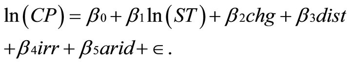 (1)
(1)
These variables are chosen because they affect the center pivot count in a county and have a reasonable amount of variation at the county level of aggregation; however, the estimated parameters from this equation are not the main interest of this study. What is of interest is whether any spillovers exist from the center pivot counts in neighboring studies.
4.3. The Spatial Lag Model
If spatial dependence exists in county center pivot counts, it means that the number of center pivots in each county is dependent on the number of center pivots in neighboring counties and can be represented by a spatial lag model (SAR): y = ρWy + Xβ + ε.
In this specification, a spatially lagged dependent variable, ρWy, is included as an independent variable to account for the effect of neighboring observations. In the SAR model, W is a spatial weighting matrix and ρ is a spatial autoregressive parameter that measures the strength of spatial interactions between neighbors. A statistically significant ρ implies that spillovers related to center pivot counts exist between counties. To account for spatial dependence in center pivot counts, Equation (1) is modified so that:
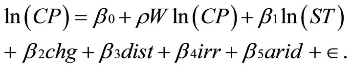 (2)
(2)
4.4. The Spatial Error Model
A second form of spatial dependence is spatial autocorrelation, or spatial dependence in the error term. When spatial autocorrelation exists, observations are grouped in such a way that measurement error depends on location. Examples of this would be if counties with high center pivot counts tended to be grouped together (positive spatial autocorrelation), or if counties with high center pivot counts tended to neighbor counties with low center pivot counts (negative spatial autocorrelation). The spatial error model (SEM) accounts for spatial autocorrelation by modifying the error term in the OLS specification, y = Xβ + ε, so that ε = λWξ + μ, where ξ is the spatially correlated part of the error term and μ ~ (0, σ2In) is spatially uncorrelated. This specification is identical to an OLS model, save for the error term, which now exhibits spatial dependence. In the SEM model, λ is a spatial autoregressive parameter that measures the strength of spatial correlation between errors, and μ is the portion of the error term that satisfies the assumptions of a normal regression model.
While spatial autocorrelation does not imply the existence of spillovers between counties, the existence of spatial autocorrelation in center pivot counts would have important implications for the diffusion of irrigation technology in this region. In this context, the presence spatial autocorrelation would imply that a county’s physical location, and perhaps its physical characteristics, is what drive the adoption decision. If this is the case then future attempts to understand the adoption decisions of producers would need to rely on a micro level approach that considers physical factors.
4.5. The Spatial Weights Matrix
Both of the spatial model specifications rely on the use of the spatial weights matrix to model spatial interaction. In the matrix, each element, wij, represents the spatial relationship between points i and j, and wij = 0 ∀ i = j. The types of weights matrices are many, and there is no formal method of choosing one method of modeling distance over another [29]. For this analysis a row standardized inverse distance matrix is used where distance, dij, is the Euclidian distance between two counties, and each element is standardized by dividing it by the number of neighbors, in this case 13, so the value of every off diagonal element is  To calculate the Euclidian distance between two counties, the geographic coordinates for the county center were taken from the Texas State Historical Society Website [30]. Assuming the geographic coordinates for two counties are the corners of a triangle adjacent to the hypotenuse, the distance between counties can be calculated using the Pythagorean Theorem.
Using the type of weighting matrix specified above assumes that all counties in the study area will have some affect on each other, but the effect will decrease as distance increases. Using a different type of weighting matrix could potentially change the nature of any spatial relationships discovered in the regression analysis. For example, using a k nearest neighbor (knn) matrix would only consider a k number of specified counties as neighbors, and only these neighbors would be considered when measuring spatial relationships. Considering the small study area, and that all of the counties included in the data are part of the same regulatory institution through membership in the HPWD, it is assumed that even individuals in the counties farthest away from each other would have some chance for contact with each other. Using an inverse distance matrix with no limit placed on distance captures these interactions.
5. Results
5.1. Correlation with Price and Interest Rate
In the analysis of aggregated spatial effects, economic variables, such as price and the interest rate, are left out because they do not vary for each observation in the cross section; thus, these variables would reduce to a fixed effect and enter the intercept during the estimation process. To examine how these variables impact the number of center pivots in a county, a regression was performed using an index of crop prices and the interest rate as independent variables. The price variable (P) is an index of the average market price reported by NASS for corn, cotton, peanuts, sorghum, and wheat. The year 1986 was used as the base and was set at 100. The interest rate (i) used was the 90 day T-bill rate. The model took the following form:
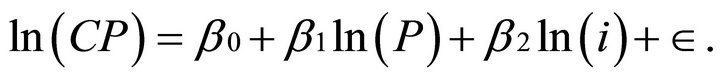 (3)
(3)
The results in Table 1 show that while these variables may be important to the individual, they have no statistically significant correlation with the aggregate level of center pivot adoption, thus confirming that omission of these variables from subsequent regressions will not result in omitted variable bias on the basis of interest rates and prices.
5.2. Exploratory Analysis
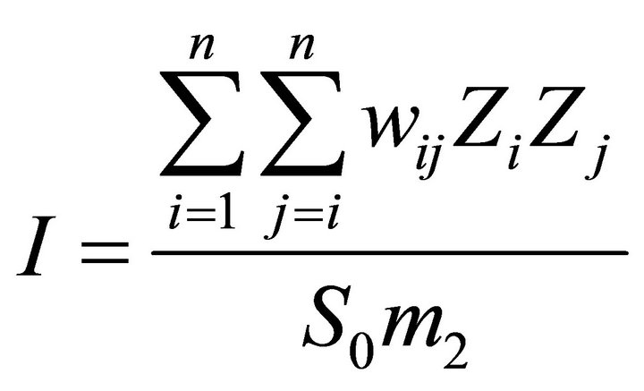
To confirm the existence of spatial clustering in center pivot numbers, a global Moran’s I test statistic was calculated for the dependent variable in each cross section. This test, proposed by [31] examines whether or not the distribution across space of observations with similar values for a variable of interest is random or not. The Moran’s I statistic is a value of global spatial autocorrelation which is calculated as
 (4)
(4)
where wij is an element of the weighting matrix,  , Yi is the value of the variable of interest at location i,
 ![]() is the mean of the variable of interest,
is the mean of the variable of interest,  , and
, and . The statistic is compared to the expected value of I,
  using a z-score, and a positive I value implies positive autocorrelation. The I statistic for each cross section is reported in Table 2.
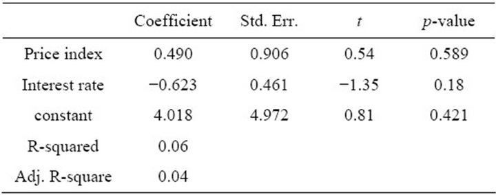
Table 1. Regression of price and interest rate variables on center pivot systems.
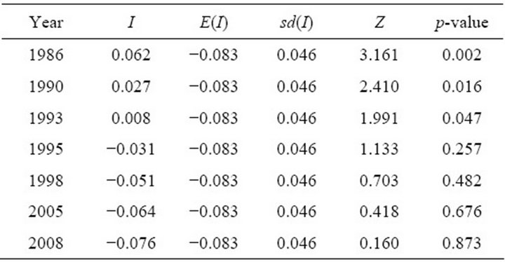
Table 2. Moran’s I values for the dependent variable (lnCP).
The Moran’s I values indicate the existence of spatial autocorrelation in only the first three cross sections. To augment the Moran’s I statistic, Moran’s scatter plots were created that give a visual representation of these results by plotting observed values of the variable of interest against the spatially lagged variable of interest. The Moran scatter plot for all years are shown in Figures 1-7. Points in the upper right quadrant indicate counties with high center pivot counts that are close to other counties with high center pivot counts. Points in the lower left quadrant indicate counties with low center pivot counts that are close to other counties with low center pivot counts.
The points of the scatter plots for the first three years have a positive skew, but the skew is decreasing from year to year. By 1995, the points are beginning to cluster more around the origin. The scatter plots for the years 1998-2008 show that the observations continue to cluster more tightly around the origin as time passes, with one exception. Randall County is an extreme outlier in the 1995-2008 scatter plots because it has the lowest number of center pivots of all the counties and is next to a county with one of the highest center pivot counts. While this may be evidence in support of dropping Randall from the rest of the analysis, the county was kept due to concerns about the already low number of degrees of freedom.
From a diffusion perspective, the reduction in spatial autocorrelation over the time period studied suggests that specific characteristics of a county determine where early adoption occurred at the individual level. In the 1986 cross section, for example, the two upper-rightmost ob-
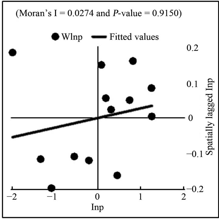
Figure 1. Moran’s scatter plot of 1986 center pivots.

Figure 2. Moran’s scatter plot of 1990 center pivots.
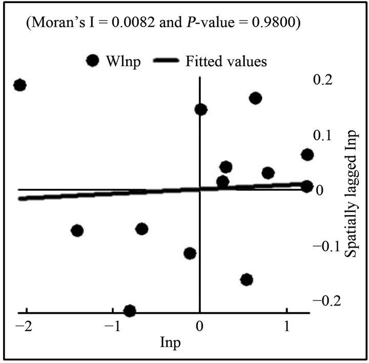
Figure 3. Moran’s scatter plot of 1993 center pivots.
servations are Bailey and Parmer counties. These two counties are situated next to each other in the region and
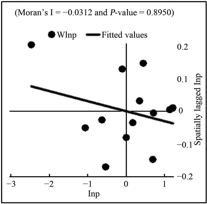
Figure 4. Moran’s scatter plot of 1995 center pivots.
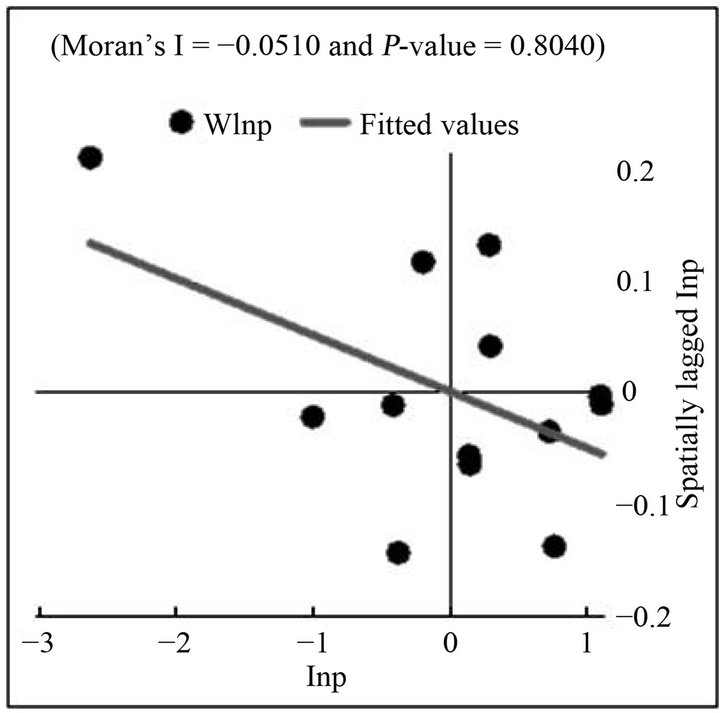
Figure 5. Moran’s scatter plot of 1998 center pivots.
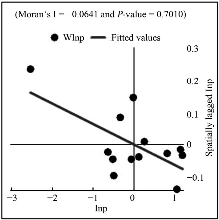
Figure 6. Moran’s scatter plot of 2005 center pivots.
also share the trait of high saturated thickness in the aquifer. If this and other traits influence individual adoption decisions are spatially located then it would make sense
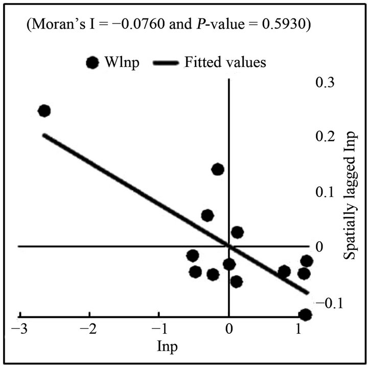
Figure 7. Moran’s scatter plot of 2008 center pivots.
for earlier years to show spatial autocorrelation, and for the autocorrelation to disappear as center pivot technology diffuses across the region.
5.3. Regression Analysis
The OLS and spatial models were estimated using STATA [32-34] for 1986, 1990, and 1993, and the results are reported in Tables 3-5. The first column in each table reports the results from the OLS regression. The second column pertains to the spatial error model (SEM) estimation and the last column reports results from the spatial lag model (SAR). At the bottom of the OLS column are the results from spatial diagnostic tests regarding the existence of spatial dependence. The first test is the Moran’s I, which is significant at the 1% level in all three of these years and indicates that the residuals from the OLS regressions exhibit spatial autocorrelation.
The Lagrange Multiplier (LM) tests listed under the Moran’s I statistic are used to determine how spatial dependence enters the model. For both spatial dependence in the error term and spatial dependence in the dependent variable, two test statistics are listed. A weakness of the standard LM tests is that the LM test for λ responds to a non-zero ρ, and the LM test for ρ responds to a non-zero λ [35,36]. The robust tests are meant to correct for this, but are only meaningful when the standard tests are significant [36].
In contrast to the Moran’s I statistic, the LM tests fail to reject the null hypothesis of no spatial dependence in either the error term or the dependent variable. To verify this result the SEM and SAR models were estimated for all three years, and Wald and LM tests run for λ = 0 and ρ = 0. The difference in results between the Moran’s I statistic and the LM test for spatial dependence in the error term is an interesting result. It would seem that when one is significant the other should be as
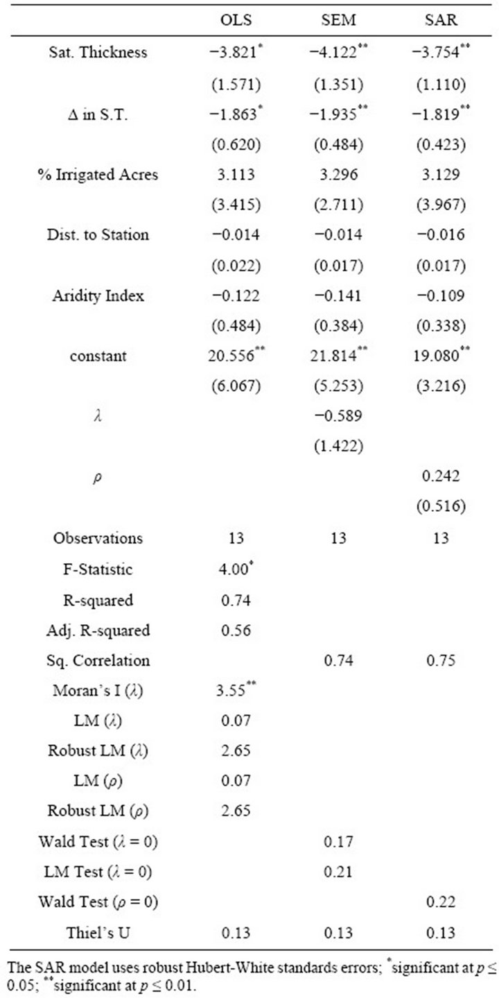
Table 3. Regression results for the 1986 cross section.
well. One possible explanation may be that the spatial clustering in the HPWD simply does not affect the error term, either because of the small size of the area or for some other unknown reason. Ultimately, however, the existence or lack thereof of spatial autocorrelation is of secondary importance. The goal of the analysis is to identify spatial spillovers. The results for these three counties make it impossible to reject the null hypothesis of no spatial dependence in the dependent variable; therefore the conclusion is that for these years there are no spillovers present.
While global Moran’s I statistics showed no sign of spatial autocorrelation in the last four cross sections,

Table 4. Regression results for the 1990 cross section.
OLS models were estimated to confirm these results, the results of which are listed in Table 6. For the years 1995 – 2005 the results are what would be expected based on the exploratory analysis; however, the Moran’s I for spatial autocorrelation in the residuals in 2008 is significant at the 5% level. Estimating the SEM and SAR models, the results of which can be found in Table 7, produce similar findings as in earlier years, and no evidence of spatial dependence was found.
6. Discussion and Conclusions
This study measures the level of spatial dependence in the number of center pivots in existence in the HPWD
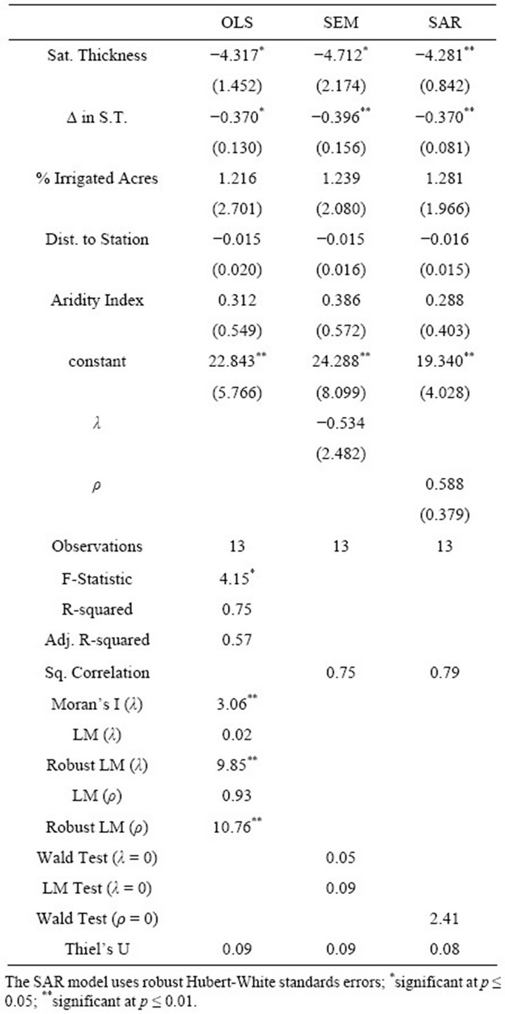
Table 5. Regression results for the 1993 cross section.
area using spatial econometric methods. The results indicate that while center pivot technology is certainly clustered spatially, at least in the earlier years of the study, there is no evidence of spatial interdependence in either the dependent variable or the error term in any of the seven cross sections studied.
This curious result may be a consequence of the small size of the study area. With only a few counties to be neighbors with, it is likely that counties with high center pivot values can be clustered together and still be near neighbors to counties with low center pivot values simply because of aquifer characteristics. One way to deal with this might be use a different weighting matrix, such
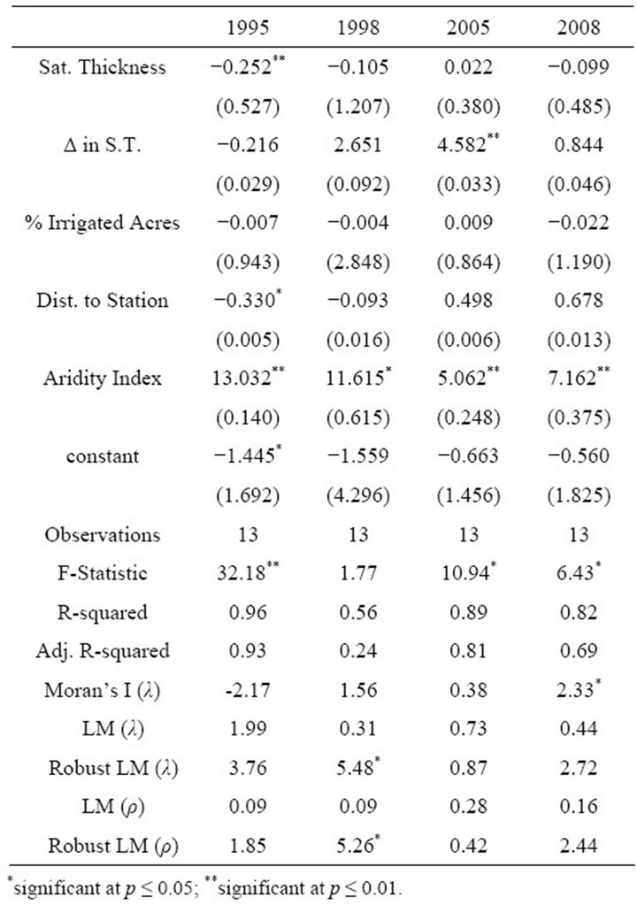
Table 6. OLS estimates for the 1995, 1998, 2005, and 2008 cross sections.
as a binary weights matrix that defines neighbors as only those observations within a critical distance, or a k nearest neighbor (knn) matrix that defines neighbors as only the k nearest observations.
Another explanation for the inability of the models to detect spatial dependence is the existence of an extreme outlier in Randall County. This would be especially true for the detection of spatial autocorrelation, which Moran’s I statistics detected in 1986, 1990, and 1993. Again, though, the small sample size becomes a problem. While dropping Randall County out of the data set might remove an outlier, it also removes an observation.
With only thirteen observations the degrees of freedom in the model is very restricting. The problem is finding data for enough observations in the same time period. The ideal data set would provide information on the irrigation adoption decisions of individuals; however, if the goal is to model spatial dependence then collecting data for enough neighboring individuals for even one time period would be a daunting task.
Two options that might improve this analysis in the future would be to either analyze the study as a panel or to reduce the number of independent variables. Taking the data as a panel would increase the number of obser-

Table 7. SEM and SAR results for the year 2008.
vations, but the semiannual center pivot counts make panel estimation difficult. Reducing the number of independent variables would free up some degrees of freedom, but in an aggregate level study that is already ignoring a number of micro level variables, what should be dropped?
It might be interesting to develop an index variable that takes into account all of the pertinent physical characteristics of a region, which would reduce the number of independent variables to one. Reducing the number of independent variables would also make the estimation of the Spatial Durbin Model (SDM) possible. The SDM was originally proposed as a means of addressing omitted variables in spatial studies. The SDM lags both the dependent variable and the independent variable, so how each observation is affected by the independent variables is different based on location. In this study, however, the SDM would have thirteen observations and eleven parameters. An index variable would reduce the number of parameters to three and make estimation more appealing.
Ultimately, the results of this study make it clear that while there is some sort of spatial relation, data limitations make understanding this relationship difficult. If patterns of spatial dependence in the adoption of irrigation technology on the Texas High Plains are important from either an academic or a policy making viewpoint, the analysis will need to make use of either different or more refined methods than those used here.
7. Acknowledgements
The authors would like to thank the Ogallala Water Project (United States Department of Agriculture, Agricultural Research Service) for their funding of this project.
We would also like to thank the staff of the High Plains Underground Water Conservation District no. 1 for their assistance with gathering data necessary for this paper.
Finally, A. Wright would like to thank Dr. Eduardo Segarra and Dr. Aaron Benson of Texas Tech University for their contributions to this research.
REFERENCES
- M. Caswell and D. Zilberman, “The Effects of Well Depth and Land Quality on the Choice of Irrigation Technology,” American Journal of Agricultural Economics, Vol. 68, No. 4, 1986, pp. 798-811. doi:10.2307/1242126
- R. Shrestha and C. Gopalakrishnan, “Adoption and Diffusion of Drip Irrigation Technology: An Econometric Analysis,” Economic Development and Cultural Change, Vol. 41, No. 2, 1993, pp. 407-18. doi:10.1086/452018
- A. Abdulai and W. Huffman, “The Diffusion of New Agricultural Technologies: The Case of Crossbred-Cow Technology in Tanzania,” American Journal of Agricultural Economics, Vol. 87, No. 3, 2005, pp. 645-59. doi:10.1111/j.1467-8276.2005.00753.x
- P. Koundouri, C. Nauges and V. Tzouvelekas, “Technology Adoption Under Production Uncertainty: Theory and Application to Irrigation Technology,” American Journal of Agricultural Economics, Vol. 88, No. 3, 2006, pp. 657-670. doi:10.1111/j.1467-8276.2006.00886.x
- G. Green, D. Sunding, D. Zilberman and D. Parker, “Explaining Irrigation Technology Choices: A Microparameter Approach,” American Journal of Agricultural Economics, Vol. 78, No. 4, 1996, pp. 1064-1072. doi:10.2307/1243862
- E. Mansfield, “Technical Change and the Rate of Imitation,” Econometrica, Vol. 29, No. 4, 1961, pp. 741-766. doi:10.2307/1911817
- F. Bass, “A New Product Growth for Model Consumer Durables,” Management Science, Vol. 15, No. 5, 1969, pp. 215-227. doi:10.1287/mnsc.15.5.215
- P. Geroski, “Models of Technology Diffusion,” Research Policy, Vol. 29, No. 4-5, 2000, pp. 603-625. doi:10.1016/S0048-7333(99)00092-X
- B. Wejnert, “Integrating Models of Diffusion of Innovations: A Conceptual Framework,” Annual Review of Sociology, Vol. 28, No. 1, 2002, pp. 297-326. doi:10.1146/annurev.soc.28.110601.141051
- E. Rogers, “Diffusion of Innovations,” 5th Edition, Free Press, New York, 2003.
- N. McRoberts and A. Frank, “A Diffusion Model for the Adoption of Agricultural Innovations in Structured Adopting Populations,” Working Paper No. 29, Land Economy Research Group, 2008. http://ageconsearch.umn.edu/handle/61117
- G. Feder, R. Just and D. Zilberman, “Adoption of Agricultural Innovations in Developing Countries: A Survey,” Economic Development and Cultural Change, Vol. 33, No. 2, 1985, pp. 255-298. doi:10.1086/451461
- A. Foster and M. Rosenzweig, “Microeconomics of Technology Adoption,” Center Discussion Paper No. 984, Economic Growth Center, Yale University, 2010. http://www.econ.yale.edu/growth_pdf/cdp984.pdf
- K. Fuglie and C. Kascak, “Adoption and Diffusion of Natural Resource Conserving Technology,” Review of Agricultural Economics, Vol. 23, No. 2, 2001, pp. 386-403. doi:10.1111/1467-9353.00068
- S. Davies, “The Diffusion Process of Innovations,” Cambridge University Press, Cambridge, 1979.
- R. Just, D. Zilberman and G. Rausser, “A Putty Clay Approach to the Distributional Effects of New Technology under Risk,” In: D. Yaron and C. Tapiero, Eds., Operations Research in Agriculture and Water Resources, North-Holland Publishing Co., Amsterdam, 1980, pp. 97- 121.
- G. Feder and G. O’Mara, “Farm Size and the Adoption of Green Revolution Technology,” Economic Development and Cultural Change, Vol. 30, No. 1, 1981, pp. 59-76. doi:10.1086/452539
- F. Shah, D. Zilberman and U. Chakravorty, “Technology Adoption in the Presence of an Exhaustible Resource: The Case of Groundwater Extraction,” American Journal of Agricultural Economics, Vol. 77, No. 2, 1995, pp. 291- 299. doi:10.1086/452539
- W. Keller, “Are International R&D Spillovers Trade Related? Analyzing Spillovers among Randomly Matched Trade Partners,” European Economic Review, Vol. 42, No. 8, 1998, pp. 1469-1481. doi:10.1016/S0014-2921(97)00092-5
- W. Keller, “The Geography and Channels of Diffusion at the World’s Technology Frontier,” NBER Working Papers No. 8150, National Bureau of Economic Research, 2001. http://www.nber.org/papers/w8150.pdf
- M. Abreu, H. Groot and R. Florax, “Spatial Patterns of Technology Diffusion,” Tinbergen Institute Discussion Paper, TI-2004-079/3, 2004. http://www.tinbergen.nl/discussionpapers/04079.pdf
- High Plains Water District No. 1, “The Cross Section,” Various Issues, 1981-2005.
- High Plains Water District No. 1, “Personal Communication, Personal Communication Regarding the Number of Center Pivots Systems in the Water District in Various Years,” 2012.
- Texas Tech University Center for Geospatial Technology, “Texas County Water Information,” 2010. http://www.gis.ttu.edu/OgallalaAquiferMaps/
- US Department of Agriculture, National Agricultural Statistics Service, “Quick Stats: US and All States County Data-Crops,” 2010. http://www.nass.usda.gov/QuickStats/Create_County_All.jsp
- S. Stadler, “Aridity Indices,” In: J. E. Oliver, Ed., Encyclopedia of World Climatology, Spinger, Berlin, 2005. http://link.springer.com/referenceworkentry/10.1007/1-4020-3266-8_17/fulltext.html
- Western Regional Climate Center, “Western US Climate Historical Summaries,” 2012. http://www.wrcc.dri.edu/Climsum.html
- Federal Reserve Board of Governors, “Selected Interest Rates,” 2011. http://www.federalreserve.gov/releases/h15/data.htm
- L. Anselin, “Under the Hood: Issues in the Specification and Interpretation of Spatial Regression Models,” Agricultural Economics, Vol. 27, No. 3, 2002, pp. 247-267. doi:10.1111/j.1574-0862.2002.tb00120.x
- Texas State Historical Society, Various County WebPages, 2012. http://www.tshaonline.org/
- P. Moran, “The Interpretation of Statistical Maps,” Journal of the Royal Statistical Society, Series B (Methodological), Vol. 10, No. 2, 1948, pp. 243-251.
- P. Jeanty, “Spmlreg: Stata Module to Estimate the Spatial Lag, the Spatial Error, the Spatial Durbin, and the General Spatial Models,” 2010. http://ideas.repec.org/c/boc/bocode/s457135.html
- P. Jeanty, “Splagvar: Stata Module to Generate Spatially Lagged Variables, construct the Moran Scatter Plot, and Calculate global Moran’s I Statistics,” 2010. http://ideas.repec.org/c/boc/bocode/s457112.html
- P. Jeanty, “Spwmatrix: Stata Module to Create, Import, and Export Spatial Weights,” 2010. http://ideas.repec.org/c/boc/bocode/s457111.html
- M. Pisati, “Tools for Spatial Data Analysis,” Stata Technical Bulletin, No. 60, 2001, pp. 21-37. http://www.stata.com/products/stb/journals/stb60.pdf
- L. Anselin, “Exploring Spatial Data with GeoDa: A Workbook,” 2005. https://geodacenter.asu.edu/system/files/geodaworkbook.pdf
NOTES
1This assumes that no other changes occur in the cost and production functions due to changes in the use of other inputs, and that no changes occur in the price of the final good.