Received 28 March 2015; accepted 5 June 2015; published 9 June 2015

ABSTRACT

This article examined in detail microwave radiometer functioning algorithm with synchronously using of the two types of pulse modulation: amplitude pulse modulation and pulse-width modulation. This allows a zero-radiometer measurement method to realize when the fluctuation effect of the receiver gain and the influence of its own noise changes are minimized. A zero balance automatically maintains in radiometer. The antenna signal is indirectly determined through the signal duration that controls the pulse-width modulation. An analytical expression of the fluctuation sensitivity was obtained in a general form. From its analysis gain in sensitivity, conditions were defined by the optimizing of the radiometer input knot’s construction. Three modifications of the radiometer input knot were researched. Fluctuation sensitivity at different measurement range was determined for modification of the radiometer input knot.

Keywords:

Microwave Radiometer, Null Method of Measurement, Fluctuation Sensitivity

1. Introduction

It is well known that study of microwave appearance of various objects of earth’s surface provides fundamentally different physical self-descriptiveness than using only optical and infrared earth remote sensing [1] [2] . This fact encourages continuous development of measurement systems aimed at improving the accuracy and the increasing of informative sensing saturation. A development of microwave remote sensing systems with low energy consumption intended for working in natural conditions and especially on the side refers to a difficult problem. Traditional approaches often lead to mutually exclusive solutions; therefore, the implementation of stringent requirements for the microwave radiometers is impossible without searching for new approaches, methods and solutions.

Methods for stabilizing or accounting of radiometer technical parameters’ changes consist in application of different functioning methods. Among various schemes, modulation radiometers have been widely used [3] [4] . These radiometers are based on method of differential measurements. At the entrance, before radiometric receiver, modulation is generated with a certain frequency antenna signal and a stable reference noise generator signal―the antenna simulator connected to the input of the receiver, instead of the antenna. Because measurements are transferred to a higher frequency with which signals are modulated, the influence of two major destabilizing factors reduces: the influence of anomalous fluctuations of the gain near zero frequency significantly decreases; constant and quasi constant of self-noise components of the radiometer decrease. Wide application of modulation radiometers is associated with a satisfactory accuracy of measurements, which is achieved essentially by simple methods (modulation at the entrance and demodulation―synchronous detection―at the output) and a simple circuit implementation. Modulation radiometers are attracted by simple design; therefore, they are promising for repeating. This is manifested in their massive using. However, the full minimizations of effect of changes of amplifier gain and self-noise of receiver in modulation scheme do not happen. It is useful noticeably to minimize these changes by using the zero method of measurement in modulation radiometer. This method has the highest potential facilities to create precision radiometers.

Ryle and Troitsky are the authors of the conception and interpretation of zero method applying to radiometers [5] [6] . A number of successful researches have associated with the creation of zero-radiometer. These researches are proof of the Nyquist formula for spectral, fluctuating noise density of various materials’ resistance validity, and discovery of the recombination rf spectral line emitted by highly excited atoms in radio astronomy, measuring abyssal temperature of the biological objects, etc. The output power of the noise reference generator is regulated before achieving the so-called zero balance in the measuring path. The so-called zero balance is being considered established if the same signals in different half-periods of a symmetric pulse of the measuring path are passing. Therefore, feedback following network and regulated reference noise source are presenting in zero radiometer. The first zero radiometer had analog regulation principle of zero balance. In this radiometer, in input knots precision operated microwave devices, adjustable attenuators or random-noise generators with regulated input power being applied. The demands of the high linear adjusting characteristic, large dynamic range, elevated response speed of regulation for bringing the measuring system in the zero balance method were established to current knots. Errors arising from using the given elements in input blocks were not allowed to fully realize the zero measurement method advantages and zero radiometers were not widely spreading.

The creation of the pulse added noise operation in the radiometer appeared as a successful development of zero method application. This operation works on pulse-width-law [7] - [9] . In this case, the average of the half- cycle modulation power of invariable reference noise signal generator is regulated by changing of the duration of its action. This led to the simplification of the input receiving block scheme (microwave switch and noise generator), improving of the linearity of calibration radiometer equation by the simple adjustment of the reference signal.

This method of mixing the reference and measured signals (in different ways pulse-modulated) led to a considerable simplification of input block design. But this method complicated modulated signals conditioning after square-law detector. It led to an increase in measurement error. Thus, schemes of the zero radiometer with pulse added noise turned out more difficult than schemes of the ordinary modulation radiometers, and therefore they were not widely used.

In this article, a new modification of the zero functioning principle of microwave radiometers by weak signal changing was considered, and the possibility of fluctuation sensitivity and stability of these systems were analyzed.

2. The Zero Method Modification of the Signal Reception

The equality of low-energy signals at the radiometric receiver input at different half-periods of a symmetric pulse modulation is achieved by the pulse duration changing. This impulse controls the introduction of additional noise signal into the supporting or the antenna paths of modulation radiometer. Time diagrams which explain the combine modulation principle in radiometer are shown in Figure 1. The control pulse-width signal t_pws changes in the range from zero to the half-period length t_mod of main modulator work.

The signals energy equality is the condition of specified balance in radiometer. These signals enter to the receivers input at different half-periods of symmetrical modulation. In Figure 1(a), these energies are proportional to the corresponding shaded areas Q₁(t) and Q₂(t). The signals energy equality is continuously maintained

by automatic pulse-width signal duration t_pws changing of radiometer controlling system. On the diagram pulse voltage amplitudes U₁, U₂, U₃ at the receiver output are proportional to appropriate signal noise temperatures Т₁, Т₂, Т₃ at the receiver input. Proportionality constant G(t) is equal to product of gain coefficient at high and low frequencies and square-law detector transmission coefficient.

Introduce the value DQ(t) which considers the inequality of Q₁(t) and Q₂(t) and includes both a constant component DQ₀ and the fluctuating part of Dq(t)

(1)

where G(t) = G₀ + g(t), G₀―constant component, g(t)―transmission coefficient fluctuation, n₁(t), n₂(t), n₃(t)― signal Т₁, Т₂, Т₃ noise entries, which take into account their noise character; H₁(q), H₂(q), H₃(q)―pulse response characteristics of accumulative receiver filters for each of the corresponding signals.

For a long time interval it is possible to use n₁(t) = n₂(t) = n₃(t) = 0 for mean value t_pws considering even deviations of noise signal components which represent the normal static ergodic processes. Also for the transmission coefficient G(t), taking into account the statistical invariance of g(t) for a long time interval its fluctuating component can be considered equal to zero. The accumulation of signals occurs by using of three integrating RC- circuits of the first order. Pulse characteristics of these circuits are determined by the well-known relation H(q) = exp(−q/t)/t, where t is circuit time constant; t = RC.

Then for the constant component of the parameter DQ(t), using (1) write

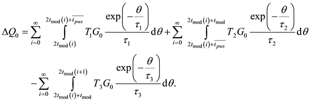(2)

It is possible to use the decomposition of exponential functions in a Maclaurin series with the two members approaching, because pulse durations t_pws and t_mod are much less than the accumulation signals time (these signals are defined by low-frequency filters constants t₁, t₂, t₃). The solution of Equation (2) is

(3)

Taking into account signal noise character and availability of the receiver amplifier gain fluctuation Q₁(t) and Q₂(t) are not equal for a modulation period. But for a large time interval in the limit for an endless number of modulation periods DQ₀ = 0 can be written due to automatic signals energy tracking system operation for uninterrupted leveling.

It results from (3) that

(4)

Solving Equation (4) relatively obtain

(5)

Equation (5) is a mathematic of the implementation of the proposed modification of the zero method reception. It follows that the antenna signal can be determined indirectly through the added noise pulse duration without signals changing in the low frequency path. Equation (5) does not include the transfer constant of the measuring path. This indicates of zero method of radiometer working.

3. Zero Method Implementation Course in Microwave Radiometers

The comparison of Q₁(t) and Q₂(t) is replaced by equivalent comparison of volt-second areas (Figure 1(b)) of positive S₁(t) and negative S₂(t) pulses at the receiver output. The pulse amplitudes are proportional to the signal differences Т₁ − Т₃, Т₃ − Т₂ at the receiver input. If the voltage of second half-period modulation is equal to zero and time zero axis passes through the Т₃ level signal, the volt-second pulse areas in the modulation first half-period are equal, S₁(t) = S₂(t) (periodic sequence). As

and

where and, then

where k―Boltzmann constant, df―frequency range band. Solving the last equation relatively obtain (5).

A sequence of simple but necessary operations follows from this reasoning. These operations must be done to transform the signals after square-law detector and low-frequency amplification. These operations are constant component exclusion in signals and voltage sign determination in the second half period of modulation. The direct component exception reduces to the pulse signal Т₃ top deflection to the zero time axis (t Þ t'). The zero balance condition (the voltage lack in the modulation second half-period on the output of the measuring tract) settles by the t_pws duration regulation. Thus antenna signal tracking is realized by the t_pws duration changing. This leads to the signal periodic sequence displacement up or down relatively the time zero axes.

4. The Fluctuation Sensitivity Analysis

DQ(t) chaotic changes in (1) are associated with the parameter Dq(t) with nonzero components n₁(t), n₂(t), n₃(t), g(t). Compute the parameter Dq(t) dispersion by correlation function method. Meanwhile take into account the statistical independence of the transmission coefficient fluctuations of the radiometer measuring path g(t) and signals Т₁, Т₂, Т₃ noise components n₁(t), n₂(t), n₃(t). The total dispersion is the sum of two dispersions. First of them allows for the receiver transmission coefficient fluctuations, the second one is caused by the noise signal nature.

The noise correlation time of function n(t) is determined by signal receiving bandwidth df and for radiometers is considerable less than modulation period 2t_mod. Consequently, these signals Т₁, Т₂, Т₃ noise components n₁(t), n₂(t), n₃(t) are uncorrelated with each other. Then the dispersion is determined from (1)

(6)

Noise n(t) autocorrelation function in comparison with pulse filters characteristics H(q) and the modulation period 2t_mod can be considered a delta function d(t) with integral value and correlation time 1/df. Accordingly, have

(7)

Exploiting (7), (6), obtain the following equation

(8)

After the replacement of (5) into (8) finally obtain

(9)

In case of equal low-frequency filters

(10)

Next determine the dispersion caused by the fluctuations of the radiometer measuring path transmission coefficient.

Write down the formula for dispersion calculating using the fundamental relation (1)

(11)

For the dispersion calculation take g(t) stationary, with a normal distribution, the exponential autocorrelation function

(12)

where is the measuring path transmission coefficient fluctuations dispersion, t₀―effective correlation time

constant of the transmission coefficient fluctuations. Typically t₀ is much greater than the radiometer accumulating filters time constants t₁, t₂ and t₃.

Compute generalized integral, through which any of the six integrals in expression (11) can be expressed. For variable arguments during the generalized integral calculating accept the conditions 2t_mod ³ x, y ³ 0; 2t_mod ³ z, v ³ 0; k,. Then

(13)

Using (13) calculate the integrals J_1g − J_6g in (11) and obtain an expression for calculating the fluctuation dispersions of the transmission coefficient

(14)

If the filters pulse characteristics are the same, obtain. A zero value of obtained dispersion indicates

on more less its value changing, than the dispersion caused by the signals noise nature. Given this dispersion of fluctuations of the transmission coefficient can be neglected. In fact an error of the dispersion determination can appear as results of the autocorrelation function approximate sampling (12), approximations for the exponential function. The received result is being coincided with the conclusions of other authors [10] [11] . These conclusions show that the zero method application allows minimizing the influence of fluctuations receivers increasing on the measurement results.

If pulse-width signal t_pws duration changing have happened at 1 time interval (discrete step), Q₁(t) changing in the first modulation half-cycle (Figure 1(a)) equal to

(15)

where N is quantity of discrete step to be placed on the half period t_mod duration. N characterizes measurements resolution.

The traditional sequence of operations is used to determine the sensitivity [12] . In the case of introduced null method measuring this traditional sequence of operations can be formulated as follows: the regulation of the pulse-width signal duration will be meaningful if this duration changing on one discrete step and associated with this volt-second areas changing of pulse signals at the receiver output in the first half-period modulation are equal to standard deviation from volt-second areas data equality. The standard deviation is caused by fluctuations and noise nature of the measuring signals. In accordance with this write

(16)

where R is a number of accumulated values of the pulse-width signal duration digital codes. There are two stages of averaging the signal in radiometers which use this modification of zero receiving method. Firstly a low-fre- quency analog signal filtering at the output of the receiver is performed. Further, in the system of added noise signal duration automatic control, except the adjustment cycle, the accumulation of digital codes of this duration with following averaging is occurring. It is known from the theory of errors; the signal dispersion is reduced

times.

After the replacement of (10), (15) into (16) obtain

(17)

Pulse-width signal duration is variated from 0 to t_mod by changing the antenna signal from minimum to maximum. Therefore for the minimum antenna signal DТ_а, which can be detected, there is a proportion

(18)

where dT_a―antenna signal measuring range, ∆t―time discrete step duration, which varies by the duration t_pws sudden change. The value of the minimum detectable antenna signal DТ_а characterizes the sensitivity.

Typically, DТ_а and dT_a are defined by the device designing. In terms of these parameters, using (18) find N. N determines the number of order n of radiometer output digital code. Using (18) the formula of radiometer fluctuation sensitivity calculation is formed from (17)

(19)

For the known radiometric receiver necessary sensitivity is achieved by selecting the t and R.

Parameter R is related to measurement time t_mes by the ratio

5. Structured Modeling of the Radiometer Input Receiving Modules

The signal modulation before their arrival at the receiver is carried out in the radiometer input block. Three signals are subjected to modulation. Two signals are reference signals Т_ref and Т_add. They are produced by reference noise generator (NG) and additional reference noise generator (ANG) accordingly. The third signal is an antenna measurable signal (А) Т_а. Combinations of these signals constitute the signals Т₁, Т₂, Т₃ on time diagrams in Figure 1. Possible signals combinations Т_ref, Т_add, Т_а for the level formations Т₁, Т₂, Т₃ are given in Table 1. Т_n?reduced to the input of the receiver self-noise effective temperature of the receiver and input block of the radiometer.

According to the received method functioning model (5) block diagrams of the three input blocks (for the respective positions of the Table 1) are shown in Figure 2. Modulator (M) alternately commutes to the receiver input or antenna signal Т_а or noise reference generator signal Т_ref. In the schemes in Figure 2(a) and Figure 2(b) additional reference signal Т_add is introduced through the microwave switch (MWS) to the antenna or supporting duct through the directional coupler (DC). Additional modulator (М₁) is introduced into the scheme in Figure 2(c).

Obtain the transfer characteristic of the radiometer for the circuit of input block in Figure 2(a) by the values of effective temperatures from Pos. 1 Table 1 substituting in Equation (5)

(20)

(t_pws duration shown without upper underlining and further averaging mark is ignored). From (20) follows that antenna signal can be determined through the pulse-width signal duration that controls the additional reference noise generator (ANG) modulation without signals change in the radiometer low-frequency part. t_pws duration is associated with antenna signal Т_а by the linear law and does not depend on the transmission coefficient of the radiometer.

Obtain antenna signal from (20) T_a = T_ref − T_addt_pws/t_mod. Define the minimum and maximum of measured signals range limit by substituting two sample extremes of the duration t_pws (equal t_mod and 0) in the last equality. T_a,min = T_ref − T_add ; T_a,max = T_ref . Where the effectives dynamic range is determined by the additional reference noise generator (ANG) signal dT_a = T_a,max − T_a,min = T_add .

The equation for sensitivity determining of radiometer with the input block Figure 2(a) can be found from (19) by substituting signals T₁, T₂, T₃ of the Pos. 1 Table 1

(21)

The radiometer measurement range dT_a with concerned input block is equal Т_add. This fact has been taken into account in equation (21).

From (21) follows that the sensitivity depends on the specific antenna signal and is variable in measurement range. In [13] , the attention was taken into the fluctuating sensitivity dependence on antenna signal. But the case of a large antenna signal was regarded in this article. Owing to super noiseless amplifier with noise floor of tens of Kelvin creation whole radiometric system self-noise were considerably reduced, which were comparable with measured signals.

Usable sensitivity occurs for the antenna signal T_a = T_ref − T_add/2 in the middle of measurement range

(22)

To achieve the necessary threshold of sensitivity during the designing of radiometer with the input block obtain the relation for product calculation from (22)

(23)

Consider t and R determination strategy by example. Let it be required to secure the measurement dynamic range 0…300 К for a receiver with noise temperature Т_n = 200 К and receiving band df = 100 MHz. It is required to provide a minimum signal-detection threshold 0.05 К (= 0.05 К) in this range. The modulating frequency in radiometer is 1 kHz (t_mod = 500 ms).

Firstly determine the levels of reference signals Т_ref = Т_а,max = 300 К, Т_add = Т_ref - Т_а,min = 300 К.

Then using (23) find.

Choose t = 30t_mod = 0.015 s to ensure the necessary dynamic properties of the regulatory system. Whence R = 1.045/t = 69. Then, for the modulation period 1 ms, the measurement time will be 69 ms.

To provide the necessary sensitivity the required capacity of radiometer output digital code is determined by further calculations. Find the number of minimum antenna signal values on the measurement range N = dT_a/DT_a,max = 6000 (consider that for a given input block structure a measurement range dT_a = Т_add). Then a rates number of radiometer output digital code n = log₂N = log₂6000. Get code size n = 13 by rounding up the whole.

Using similar calculations for other input blocks in Figure 2(b) and Figure 2(с), it is useful to get the necessary data for a modified zero-radiometer designing.

As example of sensitivity calculations by Formula (29) determine which is situated in its denominator. characterizes radiometer receiver and signal processing at low frequency. Choose radiometer

parameters as more typical: df = 100 MHz, modulation frequency 1 kHz, time constant of low frequency filter t =30ms, R = 1000 which correspond to signal time storage equal to 1 second. is dimensionless quantity equal to 78383.7. The graph in Figure 3 shows calculated by Equation (21) threshold sensitivity dependence of the modified radiometer for the most typical in remote sensing measurement ranges for a receiver with noise temperature Т_n = 50 К. These calculations imply that the sensitivity within the range of measurements remains almost invariant. At the edges of measurement range the sensitivity takes the same minimum value and insignificantly increases in the middle of the range. The sensitivity depends on the upper limit of measurement range. The minimum threshold increases in the case of range expansion in the direction of higher measurement antenna temperatures measurement.

Found by similar way: transfer characteristic, measurement range, fluctuation sensitivity of radiometer with the input blocks are tabulated in Table 2 and their schemes are shown in Figure 2(b). Calculation of minimum detectable signal for both blocks gives the same results with the same measurement ranges. The dependence of fluctuation sensitivity on antenna signal diagrams for various full scales receivers with different noise temperatures are plotted in Figure 4. The sensitivity does not remain the same in the measurement range and changes during the antenna signal modifying with almost linear variation. reaches a peak at the maximum antenna signal and trough at the antenna signal equal to minimum value of the measurement range.

For all considered input units Т_n augment leads to a proportional increase of the minimum detectable antenna signal and sensitivity deterioration occurs linearly with noise temperature increasing of the receiver and the input path.

6. Experimental Researches

The formulas obtained in section 5 for sensitivity calculations were tested in experimental researches. Sensitivity determine experiments were carried out for the considered input blocks with the radiometer at the wavelength 6.5 sm (total noise temperature of the whole system is equal to 600 K, receiving bandwidth―100 MHz, modulation frequency―1 kHz). Antenna signal changing was performed by antenna tilt variation. Directional diagram covered an area in which there were no sources of synthetic electromagnetic radiation. The sensitivity was determined for different antenna signals.

Radiometer was reconstructed and 8 series of 16 measurements with 5 minutes intervals were performed. Storage time was set equal to 1 second. Average values were calculated for each series. These values were plotted on a graph shown in Figure 5. The values of the minimum detectable antenna signal were imaged on ordinate axis; the values of the measured antenna signal were imaged on abscissa axis. Curves 1 and 2 on the graphs are constructed according to the obtained analytical dependences of the radiometer with the input blocks sensitivity calculation. Schemes of these blocks are shown in Figure 2(a) and Figure 2(c), respectively. Experimentally obtained values of sensitivity are represented by vertical lines on the given graphs. The scatter of the sensitivity measured values over standard periods of time at a constant antenna signal was taken into account. Maximum spread between findings obtained by theoretical and experimental way was about 20% with standard deviation of 8% ... 10%.

7. Conclusions

On the basis of the combined pulse modulation and the original principle of signal processing, the algorithm of the following system functioning was developed. This algorithm showed that it was useful to carry out the auto- zero balance in the radiometer by changing of pulse-width signal duration. According to this algorithm, at the output of the radiometer after constant component exclusion in the first half-period of rectangular symmetrical modulation pulse volt-second areas, equalization is performed.

This procedure is equivalent to the signal energies’ equalization at the radiometer receiver input at the different modulation half-periods. Zero voltage in the second modulation half period is an indicator of pulse volt- second areas’ equality. As a result, a mathematical model is found. This model establishes a linear relation between antenna effective temperature and duration of reference noise signal modulated by pulse-width-law.

The analysis of the fluctuation sensitivity of this measuring method pointed to variable sensitivity, the dependence on the measured antenna signal. Formulas for fluctuation sensitivity calculation were obtained and experimental verification was carried out for three proposed schemes of the modified radiometer input blocks with different measured signals’ range.

Acknowledgements

This work was supported by Russian Foundation for Basic Research, grants No. 13-07-98009, No. 15-07-04971.

References

- Sharkov, E.A. (2003) Passive Microwave Remote Sensing of the Earth: Physical Foundations. Springer/PRAXIS, Berlin.
- Astafieva, N.M., Raev, M.D. and Sharkov, E.A. (2006) Portret Zemli iz kosmosa. Globalnoe radioteplovoe pole. Priroda, 9, 75-86.
- Dicke, R.H. (1946) The Measurement of Thermal Radiation at Microwave Frequencies. Review of Scientific Instruments, 17, 268-275. http://dx.doi.org/10.1063/1.1770483
- Orhaur, T. and Waltman, W. (1962) Switched Load Radiometer. Public National Radio Astronomy Observatory, 1, 179-204.
- Ryle, M. and Vonberg, D.D. (1948) An Investigation of Radio-Frequency Radiation from the Sun. Proceeding of the Royal Society, 193, 98-119. http://dx.doi.org/10.1098/rspa.1948.0036
- Troitskiy, V.S., Lubina, A.G. and Zolotov, A.V. (1951) Sravnenie teplovih shumov nekotorix materialov nulevim metodom. Dokladi Akademii Nauk SSSR, 4, 583-586.
- Hardy, W.N., Gray, K.W. and Love, A.W. (1974) An S-Band Radiometer Design with High Absolute Precision. IEEE Transactions on Microwave Theory and Techniques, MTT-22, 382-391.
- Lawrence, R.F., Harrington, R.F. and Higdon, N.S. (1982) Flight Test Evaluation of a Noise Injection Dicke Microwave Radiometer Employing Digital Signal Processing. IEEE MTT-S International Microwave Symposium Digest, New York, 15-17 June 1982, 90-92.
- de Maagt, P.J.I., Oerlemans, R.A.E., van Gestel, J.C.A.M. and Herben, M.H.B.J. (1992) A Novel Radiometer Receiver Stabilization Method. International Journal of Infrared and Millimeter Waves, 13, 1075-1097. http://dx.doi.org/10.1007/BF01009052
- Brown, S.T., Desai, S., Wenwen, Lu. and Tanner, A.B. (2007) On the Long-Term Stability of Microwave Radiometers Using Noise Diodes for Calibration. IEEE Transactions on Geoscience and Remote Sensing, 45, 1908-1920.
- Vlaby, F.T., Moore, R.K. and Fung, A.K. (1981) Microwave Remote Sensing. Artech House, Norwood.
- Sironi, G., Inzani, P., Limon, M. and Marchioni, C. (1990) Evaluation of Small Signals with a Differential Radiometer (with Application to Radio Observations at 2.5 Ghz). Measurement Science and Technology, 1, 1119-1121. http://dx.doi.org/10.1088/0957-0233/1/10/025
- Esepkina, N.A., Korolkov, D.V. and Pariyskiy, U.N. (1973) Radioteleskopi i radiometri. Nauka, Moscow, 415 p.