Journal of Applied Mathematics and Physics
Vol.03 No.10(2015), Article ID:60527,9 pages
10.4236/jamp.2015.310152
Efficient Approach for 3D Stationary Optical Solitons in Dissipative Systems
A. Konaté, E. Soro, O. Asseu, A. Kamagaté, P. Yoboué
Ecole Supérieure Africaine des Technologies d’Information et de Communication (ESATIC), Abidjan, Cote d’Ivoire
Email: oasseu@yahoo.fr, alkamagate@gmail.com
Copyright © 2015 by authors and Scientific Research Publishing Inc.
This work is licensed under the Creative Commons Attribution International License (CC BY).
http://creativecommons.org/licenses/by/4.0/


Received 12 September 2015; accepted 20 October 2015; published 23 October 2015
ABSTRACT
We feature the stationary solutions of the 3D complex cubic-quintic Ginzburg-Landau equation (CGLE). Our approach is based on collective variables approach which helps to obtain a system of variational equations, giving the evolution of the light pulses parameters as a function of the propagation distance. The collective variables approach permits us to obtain, efficiently, a global mapping of the 3D stationary dissipative solitons. In addition it allows describing the influence of the parameters of the equation on the various physical parameters of the pulse and their dynamics. Thus it helps to show the impact of dispersion and nonlinear gain on the stationary dynamic.
Keywords:
Dissipative Solitons, Dispersion, Nonlinear Gain, Collective Variables Approach, Complex Cubic-Quintic Ginzburg-Landau Equation, (3D) Three-Dimensional Soliton, Spatio-Temporal Pulses

1. Introduction
Soliton dynamic is one of the most exciting areas of research in nonlinear optics. Different phenomena such as nonlinear gain, the saturable losses, the dispersion and others effects are crucial to dissipative solitons formation. The interaction between these different physical manifestations leads to a rich variety of structures [1] . The dissipative soliton is a typical example and its properties differ from those of conservative systems. First and foremost dissipative soliton solutions are fixed and the shape, width, amplitude are all fixed and defined by the parameters of the system rather than by the initial condition [2] . Afterwards, dissipative solitons have an internal energy exchange mechanism, whenever the energy supply is stopped; they “stop living”. So dissipative solitons only exist when there is a continuous energy supply to the system. All these properties make them attractive objects for research and their study has recently been renewed interest leading to an impressive number of works in several fields of nonlinear science [3] .
In dissipative system, the extent of the solutions is remarkably large and a variation of the parameters of the system changes the types of solutions via bifurcations. As there are several parameters in the equation, the number of solutions and bifurcations can really be enormous.
Dissipative systems in nonlinear optics admit stable solitons in one, two, and three dimensions [4] . Recent numerical studies of dissipative solitons in case of the (1D) one-dimensional showed new type of localized waves [5] -[7] and observed experimentally [8] in lasers cavities. For (1D) one-dimensional and (2D) two di- mensional solitons, the properties and conditions of their existence have been studied extensively. The (3D) three-dimensional case is still mainly in its early stages. The lack of general analytical solutions for the 3D dissipative solitons leads us to the necessity of using simple approaches to explore the existence of certain class of solutions. Indeed solving numerically a (3D) equation for a given set of parameters and a given initial condition is an extremely lengthy and costly procedure, which can take up several days in a standard PC. In this context, it is important to develop theoretical tools that can perceive soliton solutions more efficiently and envisage their domains of existence. One of the low-dimensional approximations that can be used for finding dissipative solitons is the method of moments, combined with the use of simple trial functions. Recently, we have demonstrated that the collective variables approach is also a useful tool and reduces significantly the computation time for predicting approximately the domains of existence of the stationary and pulsating dissipative soliton in the parameters space [9] .
This present work provides evidence for the (3D) stationary solutions of the complex cubic-quintic Ginzburg- Landau equation by the collective variables approach. The remainder of the paper is organized as follows. After introducing the governing equation, we present the collective variables approach. The steady state of the variational equations obtained by the collective variables approach is reported and analysed. Then, the findings of stationary solitons and investigating steady solutions are dealt. Finally, we summarize the main results in conclusion.
2. Materials and Methods
2.1. Complex Cubic-Quintic Ginzburg-Landau Equation Model (CGLE)
Our studies are based on an extended complex Ginzburg-Landau equation that includes cubic and quintic nonlinear terms. This equation (CGLE) is one of the universal equations used to describe dissipative systems. Many nonequilibrium phenomena, such as the generation of spatio-temporal dissipative structure in lasers [10] and soliton propagation in optical fiber systems with linear and nonlinear gain and spectral filtering (such as communication links with lumped fast saturable absorbers or fiber lasers with additive-pulse mode-locking or nonlinear polarization rotation) may all be described by the CGLE. This model includes cubic and quintic nonlinearities of dispersive and dissipative types. The quintic dissipative term in CGLE is essential to provide the stability of the optical pulse [11] . This model includes transverse operators to take into account spatial diffraction in the paraxial wave approximation.
It reflects the main physical effects that may occur in laser cavity such as dispersion, self-phase modulation, and the spectral filter the linear or nonlinear gains, and the linear and nonlinear losses. The normalized propagation equation reads:
 (1)
(1)
The optical envelope ψ is a complex function of four real variables , where t is the retarded time in the frame moving with the pulse, z is the propagation distance or the cavity round-trip number, and x and y are the two transverse coordinates.
The left-hand-side contains the conservative terms, namely  is for the anomalous (normal) dispersion propagation regime and
  which represents, if negative, the saturation coefficient of the Kerr nonlinearity. In the following, the dispersion is anomalous, and
  is kept relatively small. The right-hand-side of Equation (1) includes all dissipative terms: δ, ε, β and μ are the coefficients for linear loss (if negative), nonlinear gain (if positive), spectral filtering (if positive) and saturation of the nonlinear gain (if negative), respectively.
Dissipative terms describe the gain and loss of the pulse in the cavity.
There are distinctively different areas where different types of dissipative solitons exist. So the main task is to find a set of parameters where stationary solitons exist.
Now, to best of our knowledge, there is no analytical solution for the (3D) complex cubic-quintic Ginzburg- Landau equation. Indeed, research conducted to date use namely direct numerical simulations of the CGLE. This procedure is extremely and costly [12] . A task that is even more tedious is the mapping between the type of solution and the set of parameters of the equation.
This intensive work can be significantly reduced if we develop theoretical tools that can perceive soliton solutions more efficiently and envisage their domains of existence. A few approximate, semi-analytical methods based on various physical backgrounds were developed and applied to study nonlinear pulse propagation. Several of them make use of a trial function and its associated finite-dimensional dynamical system. Reductions to a finite-dimensional dynamical system use variational principles, the method of moments, and a collective variables approach. Our study is therefore to use the collective variables approach to find a rich variety of solutions that include stationary dissipative solitons of the 3D cubic-quintic Ginzburg-Landau equation.
2.2. Collective Variables Approach
The 3D cubic-quintic Ginzburg-Landau Equation (1) can be used for the description of the dynamics of ultra- short light pulses in a fiber system. However the optical field describes several phenomena like all other localized or non-localized excitations, such as noise or radiation, which are always more or less present in the real system, in addition to the pulse as a collective entity (localized in time and space).
These effects, combined with the nonlinear phenomena and dispersion chromatic lead to complex and dynamic processes particularly difficult to understand from the single solution of the propagation equation. For the best understanding of these dynamic processes, it is sometimes useful to bring the dynamics of the pulse to that of a simple physical system with only a small number of degrees of freedom. Each degree of freedom of equivalent mechanical system is associated a variable representing a physical parameter of the pulse. These variables allowing the description of pulse behavior are called collective coordinates. Mathematical methods for transforming the propagation of the pulse field equation in a system of ordinary differential equations describing the evolution of collective coordinates of the pulse during the propagation methods are called collective variables approach.
In this context, it is appropriate to simplify the characterization of the pulse by using a set of parameters (collective coordinates) that best describe the major physical characteristics of the optical pulse [13] .
The mean idea in the collective variables approach is to associate collective variables with the pulse’s parameters of interest for which equations of motion may be derived. One may introduce N collective variables, z dependent, say Xi with![]() , in a way such that each of them can correctly describe a fundamental parameter of the pulse (amplitude, width, chirp, …) [14] . To this end, one can decompose the field
, in a way such that each of them can correctly describe a fundamental parameter of the pulse (amplitude, width, chirp, …) [14] . To this end, one can decompose the field ![]() in the following way:
in the following way:
![]() (2)
(2)
where ![]() is a correction term to add to the ansatz function f to get the exact field ψ. This remedial field
is a correction term to add to the ansatz function f to get the exact field ψ. This remedial field ![]() [14] is a residual field that represents all other excitations in the system (noise, radiation, dressing field, etc.).
[14] is a residual field that represents all other excitations in the system (noise, radiation, dressing field, etc.).
The function ψ is unknown a priori; the choice of ansatz function f will ultimately be arbitrary. However this function must be selected to best represent the exact field profile ψ. The choice of the ansatz function is important for the success of the technique, especially when approximations are made.
As part of our study (as is the case in a number of interesting case studies), we can consider that the profile of the optical pulse is close to a Gaussian![]() . In that situation q = 0, this approximation is called the bare approximation [14] . In this way one can consider the fact that the pulse propagation can be completely characterized that the ansatz function, for example in optical fiber transmission systems.
. In that situation q = 0, this approximation is called the bare approximation [14] . In this way one can consider the fact that the pulse propagation can be completely characterized that the ansatz function, for example in optical fiber transmission systems.
To gain a better understanding of the dynamic processes which affect the behavior of the pulse during propagation, we will approach the optical field ψ of Equation (1) by ansatz function that can easily be expressed in terms of physical parameters of the pulse. Thus, the propagation of the pulse field equation is transformed into a system of ordinary differential equations (ODEs) describing the evolution of the parameters of the pulse during the propagation. The asset of that way is that, the ordinary differential equation can be solved numerically with relative ease. The success of this theory is based on the choice of the ansatz function, so its precise form that introduces the collective variables is rather crucial.
Recently we have demonstrated with different ansatz functions in [9] that the collective variables approach is a useful tool for predicting approximately the domains of existence of stable light bullets in the parameter space of the cubic-quintic Ginzburg-Landau equation, that give us confidence in our collective variables method. In this earlier study, the Gaussian ansatz function admits symmetrical shape of the pulse in the (x, y) plane. Drawing on the preliminary results in [9] and in order to describe more complex asymmetric deformations of the pulse in the (x, y) plane, we choose for this study, the following test Gaussian function:
![]() (3)
(3)
A, wt, wx, wy, ct, cx, cy and p represent the collective variables. With t, x and y, the temporal and transverse variables along x and y axis respectively. A stands for soliton amplitude, wt the temporal width along t, wx the transverse width along x axis and wy the transverse width along y axis. ct represents the temporal chirp parameter, cx the transverse chirp along x, cy the transverse chirp along y and p is the global phase that evolves along with propagation. When a stationary regime is reached, the phase becomes a linear function of the propagation distance z.
After choosing the ansatz function which is done according to the master Equation (1) and the type of solutions pursued, we pursue the process of characterization of the pulse by neglecting the residual field. Applying the bare approximation to the 3D CGLE, that is, substituting the field ψ by the given ansatz function ![]() and projecting the resulting equations in the following direction
and projecting the resulting equations in the following direction
![]()
we get easily the eight collective variables evolve according to the following set of eight coupled ordinary differential equation:
![]() (4)
(4)
The variational equations allow seeing clearly the influence of each Equation (1) parameters on the various physical parameters of the soliton. As well they give us the first idea on the dynamic of the light pulse. However they give no explicit information with regard to the different solutions of the Equation (1) and their stability.
The variational equations are usually functions of time that evolve subject to the constraints of the system and finally converge to fixed point or a limit cycle. A meticulous analysis of the variational equations show that the evolution of the amplitude (A) is dominated by the linear loss (δ), the nonlinear gain (ε) and its saturation (μ), as well as that the terms of spectral filtering (β) and dispersion term (D). This confirms quite well that the perfect balance between losses and gains is required to maintain the shape and stability of the soliton. The temporal (wt) and spatial widths (wx, wy) also depend on the nonlinear gain (ε) and its saturation (μ). As expected, the terms of spectral filtering (β) and dispersion term (D) affect the temporal width. As well the spatial parameters cx, cy and temporal parameters ct are influenced in the same way by the Kerr term saturation of the optical nonlinearity ( ), but the temporal term is also affected by the terms of spectral filtering (β) and dispersion term (D). Finally, not any parameters of the soliton are influenced by (p), the global phase.
The natural control parameter of the solution as it evolves is the total energy Q, and one of the key benefit of the collective variables approach is that the total energy can also expressed as function of the ansatz function parameters. Here it is interesting to gain insight from this simple and useful quantity, which is defined as
 (5)
(5)
This expression shows that the total energy is strongly ruled by the amplitude (A) the temporal (wt) and spatial widths (wx, wy). Hence the strong interest of the collective variables method because it enables a clear analysis of the equations and reveals the influence of various parameters. It is important to specify that for a dissipative system, the energy is not conserved but evolves in accordance with the so-called balance equation. If the solution stays localized, the energy evolves but remains finite. Furthermore, when a stationary solution is reached, the energy Q converges to a constant value. When the optical field spreads out, the energy tends to infinity.
After the analysis of the variational equations, our motivation remains to provide a mapping of the regions of existence of stationary solutions in the parameter space of the (3D) CGLE.
2.3. Stationary Dissipative Solitons of 3D CGLE
The main task is to find a set of parameters where stationary solitons exist. Stationary solutions exist in finite regions in the parameter space, but it would be extremely difficult to map in extensor these regions in the all dimensional parameter in which we operate. As we cannot get this mapping by varying both all the parameters of the Equation (1), we fix all the parameters and change e when looking for stable localized solutions. So from the analytical results of the variational Equation (4), we carefully analyze fixed points and we study their stability. The nonlinear gain (ε) governs the existence of fixed points and is crucial to the analysis [15] . The fixed points (FPs) of the system are found by imposing the left-hand side of ordinary differential Equations (4) to be zero ( with X = A, wt, wx, wy, ct, cx, cy, p). The threshold of existence of FPs can be estimated by the relation
 .
.
If , we have in general both stable and unstable fixed points.
The stability of FPs is determined by the analysis of the eigenvalues  (j = A, wt, wx, wy, ct, cx, cy, p) of the matrix
 .
.
The stability criterion is as follows: if the real part of at least one of the eigenvalues is positive, the corresponding FP is unstable. Hence, to have stable FP, the real parts of all the eigenvalues of the matrix Mij must be negative. The stable fixed points correspond to stationary solutions of the (3D) CGLE.
When we are looking for localized structures like dissipative solitons, the initial condition must also be localized. Its exact shape is relevant but plays a secondary role if only one type of solutions exists for a given set of parameters. The shape becomes highly important when several stable solutions coexist. So here we use this initial condition:

We restrict ourselves to fix all the parameters except for two that we vary. We have chosen the dispersion D and the cubic nonlinear gain ε as the variable parameters. So for each set of parameters, we study the existence of the fixed point and its stability. Thus, by investigating the parameter regions situated in the neighborhood of the parameters μ = −0.1, δ = −0.4, β = 0.1, ν = −0.08 and γ = 1; according to our previous study [15] [16] , we find in the (D, ε) plane a rich variety of dissipative soliton of Equation (1). So for each value pair (D, ε) the Newton-Raphson provides to look for the fixed point and we study its stability. Thus one can easily map the cartography of the solution of the Equation (1).
The Figure 1 shows the mapping of the solutions for the range of selected values. This cartography represents the solutions of the 3D CGLE equation from collective variables approach. The colored domain depicts the stable fixed points, which are the basin of attractors. Near this stable points, all the others points converge. The region of the stable fixed points represents the domain of stationary solitons of 3D cubic-quintic Ginzburg-Landau Equation (1) described in Section 2 and found from semi-analytical approach. In this domain, all the solitons parameters (amplitude, width, chirp...) stay stationary throughout propagation. Above the stationary domain, we have instable fixed points which can be dived in two categories: the limit-cycle attractor and the instable solutions. But here, our main interest is to study the dynamic of the pulse in the stationary domain (colored area).
This map (Figure 1) is similar to those studied in the planes in ,
,  ,
,  and
and  [15] [16] . So according to the cubic nonlinear gain ε value for a given set for fixed values the dynamic of the solition changes, from stationary to non-stationary. In the (D, ε) plane it may be noted that stationary dissipative soliton can exist primarily in the regions of low values of the cubic nonlinear gain. Below the lower limit, the solution dissipates and eventually vanishes because the energy pumped into the system is not enough to support the solitons in this situation. Although, the energy supply inflates the soliton to the extent that it grows indefinitely when ε is above the upper value. However, between these regions there is a small intermediate region of values where stationary solutions are transformed into pulsating ones before the continuous inflating begins.
In the stationary domain (colored area), for each unique pair (D, ε) there is one and only one type of stationary soliton with its own characteristics (amplitude, widths, energy...). As illustrated in Figure 2 an example of such dissipative soliton obtained for the following parameters μ = −0.1, δ = −0.4, β = 0.1, ν = −0.08, γ = 1, ε = 0.55 and D = 1. The soliton amplitude, widths remain constant regardless of the propagation distance. However we find that the temporal width (Figure 2(b)) and spatial (Figure 2(c) and Figure 2(d)) do not have the same values during the propagation. By contrast the following two transverse widths along x and y axes have the same characteristics. These results are in line with the ordinary differential Equations (4). In this case, the soliton amplitude (Figure 2(a)) remains at a constant value but different of those widths as expected. The same applies for the total energy of the soliton we previously expressed in terms of collective coordinates. For the same parameter values as the previous Figure 2, we have followed the evolution of the total energy and get the result shown in Figure 3. We note that it remains stationary as the other parameters of the soliton. For another set of parameters in the same region, the dynamics of the 3D soliton remains the same but with different values of amplitude, widths and chirp. This behavior is similar for all physical quantities of stationary 3D dissipative soliton.
Figure 4 clearly shows the temporal profile of such stationary dissipative soliton unchanged regardless of the propagation distance. Always to the same values, the transverse profile is also shown in Figure 5 with the same characteristics.

Figure 1. Cartography of stationary (color domain) dissipative solitons found from collective variables approach in the (D, ε) plane using the Gaussian trial function. Other CGLE parameters appear inside the figure.

Figure 2. The evolution of the following collective variables with respect to z is shown: (a) the amplitude, (b) the temporal width, (c) the width along the x axis and (d) the width along the y axis. μ = −0.1, δ = −0.4, β = 0.1, ν = −0.08, γ = 1, ε = 0.55 and D = 1.

Figure 3. Evolution of the total energy of the stationary dissipative soliton. μ = −0.1, δ = −0.4, β = 0.1, ν = −0.08, γ = 1, ε = 0.55 and D = 1.

Figure 4. Evolution of the temporal profile of the stationary dissipative soliton. μ = −0.1, δ = −0.4, β = 0.1, ν = −0.08, γ = 1, ε = 0.55 and D = 1.
As we have seen, the cubic nonlinear gain ε parameter is very important in the dynamics of dissipative system especially in the 3D case. It conditions the existence of stationary solutions and has great influence on their propagation.
The higher the cubic nonlinear gain value is set, the dissipative solitons become even more powerful with more energy. This analysis is illustrated by Figure 6. Indeed we have chosen three values (0.52, 0.55, and 0.57) of ε in the stationary domain. First, we note that according to the value of the dispersion, the total energy variation is quasi-linear and increases as the parameter D. Finally as shown in Figure 7 for ε greater, the soliton
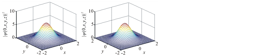
Figure 5. Transverse profile of the stationary dissipative soliton. μ = −0.1, δ = −0.4, β = 0.1, ν = −0.08, γ = 1, ε = 0.55 and D = 1.

Figure 6. Evolution of the total energy of the stationary dissipative soliton for different values of du nonlinear gain (ε = 0.52, ε = 0.555 and ε = 0.57), for a given set of a parameters μ = −0.1, δ = −0.4, β = 0.1, ν = −0.08 and γ = 1.

Figure 7. Temporal profile of the stationary dissipative soliton for different values of dispersion (D = 2, D = 5 and D = 10). Other CGLE parameters appear inside the figure.
energy becomes large leading in more complex dynamics. This explains part of the unstable solutions when we exceed the critical value of ε, in that the very high energy leads to an “explosion” of the dissipative soliton after pulsating (stable limit cycles).
The Figure 8 represents the evolution of the spatial profile along x and y axis soliton for different values of the dispersion (D = 2, D = 5 and D = 10 ), but keeping the other parameters. It merged from the analysis of the Figure 8 that the spatial widths of the soliton remain unchanged when the dispersion (D) value increases.

Figure 8. Transverse profile of the stationary dissipative soliton for different values of dispersion (D = 2, D = 5 and D = 10). Other CGLE parameters appear inside the figure.
The terms  and
and  of the ordinary differential equations which are independent of the dispersion, confirm this dynamic. In contrast, we note that in these cases the amplitude increases very slightly. These figures clearly illustrate the fact that the dispersion does not act the spatial profile but only on the temporal profile of the soliton as explicitly show the ordinary variational equations. Thus, thanks to the master equations from collective variables approach, we obtain a clear understanding of the consequence of the evolution of different pamareters on the 3D optical soliton.
3. Conclusions
In conclusions, based on collective variable approach, we have presented the cartography of stationary dissipative solitons modeled by the 3D complex cubic-quintic Ginzburg-Landau equation. We showed that the stationary soliton in this model can be regarded with asymmetric deformations of the pulse in the (x, y) plane. In particular, for a suitable choice of the ansatz function and the parameters, we have highlighted the evolution of physical parameters (amplitude, width…) of the soliton and analyzed their dynamics. Thus we investigated the influence of the dispersion parameter on the spatial and temporal profile of the 3D soliton.
We showed that the dynamics of soliton can be controlled by the choice of the system parameters. So according to the values of the nonlinear gain, the soliton energy becomes large leading in more complex dynamics. It appears quite clear that the collective variables approach is very efficient for approximating stable stationary solutions when a suitable trial function is chosen. And this technique is incomparably quicker than direct numerical computations.
Thus this present result can be deepened by implementing other dynamics (pulsating), or confirmed by purely numerical studies. Studies on this type of solitons are useful both from the fundamental point of view and for the development of composants dedicated to the treatment with purely optical path of the guide optical pulses ultra high speed telecommunications.
Cite this paper
A.Konaté,E.Soro,O.Asseu,A.Kamagaté,P.Yoboué, (2015) Efficient Approach for 3D Stationary Optical Solitons in Dissipative Systems. Journal of Applied Mathematics and Physics,03,1239-1248. doi: 10.4236/jamp.2015.310152
References
- 1. Saarlos, W.V. and Hhenberg, P.C. (1992) Fronts, Pulse, Sources and Sinks in Generalized Ginzburg-Landau. Physica D, 56, 303-367.
http://dx.doi.org/10.1016/0167-2789(92)90175-M - 2. Akhmediev, N. and Ankiewicz, A. (2003) Solitons around Us: Integrable, Hamiltonian and Dissipative Systems. In: Porsezian, K. and Kurakose, V.C., Eds., Optical Solitons: Theoretical and Experimental Challenges, Springer, Heidelberg.
- 3. Akhmediev, N. and Ankiewicz, A. (2005) Dissipative Solitons. Springer, Heidelberg.
http://dx.doi.org/10.1007/b11728 - 4. Rosanov, N.N. (2002) Spatial Hysteresis and Optical Patterns. Springer, Berlin, Chap. 6.
http://dx.doi.org/10.1007/978-3-662-04792-7 - 5. Sakaguchi, H. and Malomed, B.A. (2001) Instabilities and Splitting of Pulses in Coupled Ginzburg-Landau Equations. Physica D, 154, 229-239.
http://dx.doi.org/10.1016/S0167-2789(01)00243-3 - 6. Akhmediev, N., Soto-Crespo, J.M. and Town, G. (2001) Pulsating Solitons, Chaotic Solitons, Period Doubling, and Pulse Coexistence in Mode-Locked Lasers: CGLE Approach. Physical Review E, 63, Article ID: 056602.
http://dx.doi.org/10.1103/PhysRevE.63.056602 - 7. Deissler, R.J. and Brand, H.R. (1994) Periodic, Quasiperiodic, and Chaotic Localized Solutions of the Quintic Complex GinZburg-Landau Equation. Physical Review Letters, 72, 478-481.
http://dx.doi.org/10.1103/PhysRevLett.72.478 - 8. Soto-Crespo, J.M., Grelu, M.Ph. and Akhmediev, N. (2004) Bifurcations and Multiple-Period Soliton Pulsations in a Passively Mode-Locked Fiber Laser. Physical Review E, 70, Article ID: 066612.
http://dx.doi.org/10.1103/physreve.70.066612 - 9. Kamagaté, A., Grelu, Ph., Tchofo-Dinda, P., Soto-Crespo, J.M. and Akhmediev, N. (2009) Stationary and Pulsating Dissipative Light Bullets from a Collective Variable Approach. Physical Review E, 79, Article ID: 026609.
http://dx.doi.org/10.1103/physreve.79.026609 - 10. Haus, H.A., Fujimoto, J.G. and Ippen, E.P. (1995) Structures for Additive Pulse Mode Locking. Journal of the Optical Society of America B, 8, 2068-2076.
http://dx.doi.org/10.1364/JOSAB.8.002068 - 11. Moores, J.D. (1993) On the Ginzburg-Landau Laser Mode-Locking Model with Fifth-Odersaturable Absorber Term. Optics Communications, 96, 65-70.
http://dx.doi.org/10.1016/0030-4018(93)90524-9 - 12. Soto-Crespo, J.M., Akhmediev, N. and Grelu, P. (2006) Optical Bullets and Double Bullet Complexes in Dissipative Systems. Physical Review E, 74, Article ID: 046612.
http://dx.doi.org/10.1103/physreve.74.046612 - 13. Boesch, R., Stancioff, P. and Willis, C.R. (1988) Hamiltonian Equations for Multiple-Collective-Variable Theories of Nonlinear Klein-Gordon Equations: A Projection-Operator Approach. Physical Review B, 38, 6713-6735.
http://dx.doi.org/10.1103/PhysRevB.38.6713 - 14. Tchofo-Dinda, P., Moubissi, A.B. and Nakkeeran, K. (2001) Collective Variable Theory for Optical Solitons in Fibers. Physical Review E, 64, Article ID: 016608.
http://dx.doi.org/10.1103/physreve.64.016608 - 15. Soto-Crespo, J.M., Akhmediev, N. and Town, G. (2002) Continuous-Wave versus Pulse Regime in Passively Mode-Locked Laser with a Fast Saturable Absorber. Journal of the Optical Society of America B, 19, 234-242.
http://dx.doi.org/10.1364/JOSAB.19.000234 - 16. Kamagaté, A. (2010) Propagation des solitons spatio-temporels dans des milieux dissipatifs. Thesis, Universite de Bourgogne, Bourgogne.