International Journal of Intelligence Science
Vol.05 No.03(2015), Article ID:53761,11 pages
10.4236/ijis.2015.53012
Extending Qualitative Probabilistic Network with Mutual Information Weights
Kun Yue1, Feng Wang2, Mujin Wei1, Weiyi Liu1
1Department of Computer Science and Engineering, School of Information Science and Engineering, Yunnan University, Kunming, China
2Yunnan Computer Technology Application Key Lab, Kunming University of Science and Technology, Kunming, China
Email: kyue@ynu.edu.cn
Academic Editor: Prof. Zhongzhi Shi, Institute of Computing Technology, Chinese Academy of Sciences, China
Copyright © 2015 by authors and Scientific Research Publishing Inc.
This work is licensed under the Creative Commons Attribution International License (CC BY).
http://creativecommons.org/licenses/by/4.0/


Received 15 January 2015; accepted 30 January 2015; published 3 February 2015
ABSTRACT
Bayesian network (BN) is a well-accepted framework for representing and inferring uncertain knowledge. As the qualitative abstraction of BN, qualitative probabilistic network (QPN) is introduced for probabilistic inferences in a qualitative way. With much higher efficiency of inferences, QPNs are more suitable for real-time applications than BNs. However, the high abstraction level brings some inference conflicts and tends to pose a major obstacle to their applications. In order to eliminate the inference conflicts of QPN, in this paper, we begin by extending the QPN by adding a mutual-information-based weight (MI weight) to each qualitative influence in the QPN. The extended QPN is called MI-QPN. After obtaining the MI weights from the corresponding BN, we discuss the symmetry, transitivity and composition properties of the qualitative influences. Then we extend the general inference algorithm to implement the conflict-free inferences of MI-QPN. The feasibility of our method is verified by the results of the experiment.
Keywords:
Qualitative Probabilistic Network (QPN), Inference Conflict, Mutual Information, Influence Weight, Superposition

1. Introduction
Bayesian network (BN) is a well-accepted model to represent a set of random variables and their probabilistic relationships via a directed acyclic graph (DAG) [1] [2] . There is a conditional probability table (CPT) associated with each node to represent the quantitative relationships among the nodes. BN has been widely used in different aspects of intelligent applications including representation, prediction, reasoning, and so on [1] [3] . However, exact inference in an arbitrary BN is NP hard [4] , and even the approximate inference is also very difficult [5] . As a result, BN’s inferences are not very efficient, which is doomed to pose limits to BN-related applications, especially for real-time situations. Fortunately, as the qualitative abstraction of BN, QPN was proposed by Wellman [6] and can be appropriately used to remedy the above drawbacks of a BN. A QPN adopts a DAG to encode random variables and their relationships, which are not quantified by conditional probabilities, but are summarized by qualitative signs [7] . The most important thing is that there has been an efficient QPN inference (reasoning) algorithm, which is based on sign propagation and run in polynomial time [8] .
However, the high abstraction level of QPN results in the problem that there is no information left to compare two different qualitative influences in a QPN. Thus, when a node receives two inconsistent signs from its two different neighbor nodes during inferences, it is hard to know which sign is more suitable for the node, so that the “? (i.e., unknown)” sign is obtained as the result sign on the node. This means that there are inference conflicts generated on the node, which lead to less powerful expressiveness and inference capabilities than expected for real-world prediction and decision-making of uncertain knowledge in economics, health care, traffics, etc [9] - [16] . Worst of all, when the ambiguous results caused by inference conflicts are produced, they will be spread to most parts of the network with the reasoning algorithm going on.
To provide a conflict-free inference mechanism of QPN is paid much attention. Various approaches have been proposed from various perspectives. However, in some representative methods [9] [11] [13] , the original sample data or threshold values are required or predefined when the influences are weighted quantitatively. This is not consistent with the BN-based applications that focus on probabilistic inferences taking as input BN without the original sample data. Furthermore, a BN is frequently defined by experts instead of learned from data. Even though the original data are available, the efficiency of the process of deriving influence weights is sensitive to the data size. Meanwhile, the uncertainty of the influence weight has not been well incorporated, and the propagation of influence weights lacks solid theoretical foundations during QPN inferences.
Therefore, in this paper we are to consider eliminating the inference conflicts of general QPNs and developing a conflict-free inference method. We derive the quantitative QPN by adding a weight to each qualitative influence from the corresponding BN, while sample data and threshold values are not required. The weight is adopted as the information to compare two different qualitative signs. Therefore, when a node in a general QPN faces an inference conflict, a trade-off will be incorporated to avoid the conflict based on the weights.
Mutual information (MI) is a quantity that measures the mutual dependence of the two random variables [17] [18] . As well, MI is widely applied to test the association degree among the BN nodes [19] - [21] . When node A receives two inconsistent signs from its two different neighbor nodes, say B and C, we can naturally think that the result sign on A is more dependent on the sign propagated from B than that from C, if the mutual information between A and B is larger than that between A and C. Based on the above idea, we adopt MI as the weight to quantify the degree of the mutual dependence between two nodes linked by a directed edge.
Generally speaking, the main contributions of this paper can be summarized as follows:
We define the MI-based weight of a qualitative influence, called MI weight, and extend the traditional QPN by adding a MI weight to each qualitative influence. We call the extended QPN as MI-QPN.
We propose an efficient algorithm to derive MI weights from the conditional probability tables and prior probability distributions in the corresponding BN instead of the sample data.
We discuss the symmetry, transitivity and composition properties of qualitative influences in the MI-QPN. Then, we extend the general QPN’s inference algorithm to achieve conflict-free inferences with the MI- QPN.
We give preliminary experiments to verify the feasibility and correctness of our method.
2. Related Work
BN has been successfully established as a framework to describe, manage uncertainty using the probabilistic graphical approach [2] [3] . As the qualitative abstraction of BN, QPN [6] was proposed by Wellman and widely used in decision making, industrial control, forecasting, and so on [22] - [24] . The methods to construct QPNs mainly include deriving QPNs from the corresponding existing BNs [15] or giving QPNs by the domain experts. As for the QPN’s inference, an efficient algorithm was proposed by Druzdzel et al. [8] . The inference conflict has become a common problem for QPNs and how to resolve the inference conflicts is the subject that was paid much attention in recent years. Various methods were proposed from various perspectives.
Lv et al. [9] proposed the ambiguity reduction method by associating a qualitative mutual information weight to each qualitative influence in the QPN, but the weight can only be obtained from the given or generated sample data. This is not always feasible, since the BN may be not learned from data, or the sample data cannot be available. Parsons [10] introduced the concept of categorical influence, which is either an influence that serves to increase a probability to 1 or an influence that decreases a probability to 0, regardless of any other influences. By this approach, only some of the inference conflicts can be resolved.
Renooij et al. [11] [15] proposed two methods to solve the inference conflicts by using both kappas values and pivots to zoom upon inferences. The kappas value based method distinguishes the strong and weak influences by the interval values that do not have solid theoretical basis for interval value propagation during QPN inferences. Renooij et al. [12] presented an enhanced QPN that differs from a regular QPN to distinguish between strong and weak influences. This method is only suitable for the binary-variable situation. A threshold value is required in these methods except that exploits context-specific information. Renooij et al. [13] proposed SQPN (semi-QPN) by associating a probability interval value with each qualitative influence to quantify the qualitative influences. De Campos et al. [25] discussed the complexity of inferences in polytree-shaped SQPNs. Renooij et al. [14] extended QPNs by providing the inclusion of context-specific information about influences and showed that exploiting this information upon inference had the ability to forestall unnecessarily weak results. By this method, a threshold value should be given to distinguish the strong and weak influences.
We extended QPN to solve inference conflicts by adding the weights to qualitative influences based on the rough set theory and interval probability theory respectively in [16] and [26] . By the method in [16] , the dependency degree was computed based on the threshold value, but the corresponding sample data was required to obtain the weights. By the method in [26] , the interval-probability weights were derived from the corresponding BN’s CPT, but the calculation of interval probability during inferences led to approximate results.
3. Preliminaries and Problem Statement
3.1. The Concept of QPN
A QPN has the same graphical structure as the corresponding BN, also represented by a DAG. In a QPN, each node accords with a random variable, and the influence between each pair of the nodes can only be one of the signs including “+”, “−”, “?” and “0”, where “+” (“−”) means the probability of a higher (lower) value for the corresponding variable increases, sign “?” denotes the unknown influence by giving an evidence and “0” represents initial state of the variable without observations. Each edge with a qualitative sign means the qualitative influence between two corresponding variables. The definition of the qualitative influence [6] is given as follows.
Definition 3.1 We say that A positively influences C, written , if for all values
 ,
,
 and x, which is the set of all of C’s parents other than A,
 .
.
This definition means the probability of a higher value of C is increased when given a higher value of A, regardless of any other direct influences on C. A negative qualitative influence S− and a zero qualitative influence S0 are defined analogously, by replacing ³ in the above formula by £ and = respectively. If the qualitative influence between A and C does not belong to the above three kinds, written .
.
Example 3.1 Based on Definition 3.1 and from the BN shown in Figure 1, we derive a QPN shown in Figure 2.
3.2. QPN Inference and Inference Conflicts
It is known that the qualitative influence of a QPN exhibits various useful properties [6] . The symmetry prop-
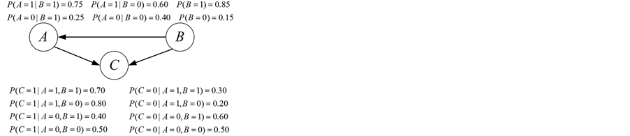
Figure 1. An simple BN.
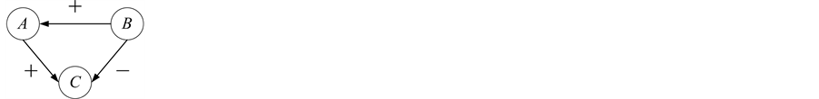
Figure 2. QPN derived from the BN in Figure 1.
erty expresses if there is
 in a QPN, then we have
 . The transitivity property can be used to combine qualitative influences along a trail without a head-to-head node into a single influence with the Ä- operator. The composition property asserts that multiple qualitative influences between two nodes along parallel chains combine into a single influence with the Å-operator. The ambiguous results (“?”) maybe appear by Å- operator during inference, and then will be propagated to other nodes by Ä-operator.
Building on these three properties and operators, Druzdzel et al. proposed an efficient inference algorithm based on sign propagation [8] . The algorithm traces the effect of observing a value for one node on the other nodes by message-passing between neighbors. When the evidences are given to the network, each node receiving a message updates its sign and subsequently sends a message to each (induced) neighbor node that is independent of the observed node. The sign propagation reach all the nodes that are not d-separated with the evidence nodes. During the process of sign propagation, each node has changed its sign at most twice.
The inference conflicts take place when a node receives two different kinds of qualitative signs (“+” and “−”). In fact, the weights of qualitative influences in a QPN are not always equivalent. Thus, in this paper, we will add a weight to each qualitative influence so that a node facing a conflict will take a sign (“+” or “−”) instead of “?” by comparing the corresponding weights.
4. Constructing MI-QPN
4.1. Concepts of Mutual Information
It is well known that information entropy quantifies the information contained in a message and is a measure of the uncertainty associated with a random variable. Now we introduce relevant definition [17] and properties [1] .
Definition 4.1 The information entropy
 of a discrete random variable
 with possible values
 is
is
 (1)
(1)
Definition 4.2 The conditional information entropy of
 given
given
 is
is
 (2)
(2)
where
 and
and
 are two discrete random variables,
 ,
,
 and
and
 (or
(or ) denotes the total number of possible values of
 (or
(or ).
).
We know
 is regarded as a measure of uncertainty about a random variable
 , and
, and
 denotes the amount of uncertainty remaining about
 when
when
 is known. The mutual information is just defined as the difference between
 and
and , which is to denote the amount of uncertainty in
 that is removed by knowing
 .
.
Definition 4.3 The mutual information of two discrete random variables
 and
and
 is defined as
 (3)
(3)
4.2. Defining MI-QPN
It is known that the dependency quantity
 on
on
 is the same with that of
 on
on . However, the same dependency degree may have different influences on
 and
and
 respectively. This means that the weight of
 does not always equal that of
 , although we always have
 . Intuitively, for any node
 with two different neighbor nodes
 and
and , if the degree of the mutual dependence be-
tween
 and
and
 is greater than that between
 and
and , then the weight of
 should be greater than that of
 . Consequently, we know the weights of qualitative influences should satisfy the following properties: 1)
 does not always equal
 ; 2) For any
 ,
,
 and
and ,
,
 .
.
Now, we define the weight of a quantitative influence based on a normalized variant of the mutual information. The weight is called MI weight that satisfies the above properties.
Definition 4.4 The MI weight of a qualitative influence
 is defined as
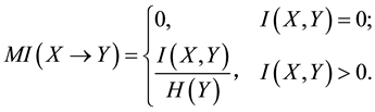 (4)
(4)
From the above definition, we know that the MI weight further satisfies the third property: 3)
 . Especially,
 when
when
 depends on
 completely, and
 = 0 when
 and
and
 are independent.
Then, we consider the concerned computation in each of the three properties of the MI weight as follows:
・ For the first property, if , we have
 . If
. If
 and
and , we know
 and
and . Thus, we have
 .
.
・ For the second property, if , we have
 , since
 . Then, we have
 (5)
(5)
since if , otherwise
 . Then, we have
 (6)
(6)
If , then we have
 (7)
(7)
If , we have
 since
since
 (8)
(8)
Therefore, the second property can be derived from Definition 4.4.
・ For the third property, if , we have
 (9)
(9)
If , we have
 (10)
(10)
Thus, we have ,
,
 and
and , and if
 , we have
 (11)
(11)
By Formulae (9), (10) and (11), we can obtain .
.
Definition 4.5 If we have , we denote the qualitative influence with an MI weight as
 , where
 .
.
By the symmetry property of the qualitative influence, we know
 implies
 . Based on Definition 4.5, we know
 . Therefore, two MI weights are added to each QPN edge to repre-
sent bidirectional qualitative influences with the MI weights between the corresponding two nodes.
Definition 4.6 MI-QPN is a DAG , where
 is a set of variables (nodes) in the graph, and
 is a set of qualitative relations and each qualitative influence in
 is associated with a MI weight.
4.3. Deriving MI Weights from BN
We can obtain a prior probability distribution from each orphans node and a CPT from each non-orphans one taking as input the BN directly. If
 is a orphans node, we denote the prior probability distribution as set
 . Otherwise, we denote the CPT of node
 with parents
 as the probability set
 , where

denotes the total number of possible states of , and
, and
 means the
 -th state of
 . It is worth noting that
 are independent given the value
 of their child node
 .
.
In order to derive the MI weights between
 and its parent

 , it is necessary to obtain the conditional probability sets associated with
 and
and , denoted as
 .
.
It is also necessary to compute the prior probability distribution of
 and
and , denoted as
 ,
, . Then, we can use
 ,
, and
and
 to compute the MI weights of the qualitative influences associated with
 and
and
 according to Definition 4.4. Let
 and
and
 be the
 -th state and the total number of possible states of random variable

 , respectively,
 . Let
. Let , if
, if , for all
 and for any
 ,we have

where
 denotes the probability of
 taking the
 -th state, given
 taking the si-th state for each

 , i.e.,
 .
.
It can be seen that we need traverse the CPT once to derive the conditional probability set associated with one node and one of its parents. With the CPTs and the prior probability distributions of a BN, we propose Algorithm 1 to compute the MI weights for each qualitative influence in the MI-QPN.
As the basic operation in Algorithm 1, the multiplication operation for computing relevant probabilities in get conditional probability is the most time-consuming operation. Let m and n be the number of non-orphans nodes and the maximal in-degree of these nodes respectively. For convenience, we suppose the number of each node’s possible values, denoted as , is the same as that in the corresponding BN. Thus, the total number of rows of each orphans node’s CPT is
 . For each orphans node, the multiplication operation can be expressed for
 times, which leads to the time complexity of Algorithm 1 in the worst case is
 . This means that to compute the MI weights for a QPN, we need scan each conditional probability table in the relevant BN for
 times at most.
Example 4.3 We consider the MI weights for the QPN in Figure 2. By Algorithm 1, we can obtain the corresponding MI-QPN shown in Figure 3.
5. Conflict-Free Inference with the MI-QPN
It is known that
 implies
 according to the symmetry property. Then, we know there exist
 in the MI-QPN by Definition 4.4, since
 exists in the corresponding QPN. We can obtain
 (12)
(12)
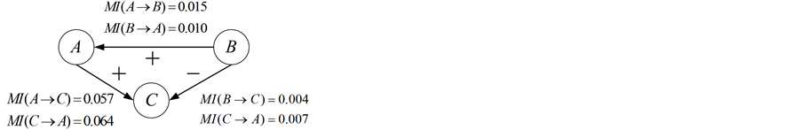
Figure 3. MI-QPN.

Algorithm 1.Deriving MI weights from a BN.
In order to address the transitivity property, we consider the MI-QPN fragment in Figure 4, where X denotes the predecessors of
 other than
 , and
, and
 represents the predecessors of
 other than
 . From this
network, we have
 and
and . Based on
 and
and , we
, we
are to derive the qualitative influence of
 on
on
 with an MI weight, denoted as
 .
.
First, based on QPN’s transitivity property, we can obtain . Then, we derive the MI weight of qualitative influence
 on
on ,
, . The transitivity property is denoted as
 (13)
(13)
In order to discuss the composition property, we consider the MI-QPN fragment in Figure 5, where X denotes
the predecessors of
 other than
 and
and . From the MI-QPN, we have
 and
and . Then, we are to derive the combination influence of
 and
and , denoted as
 (14)
(14)
where ,
,
 denotes the composition weight and “Ú” is the composition operator.
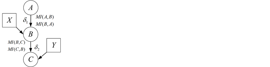
Figure 4. MI-QPN fragment.
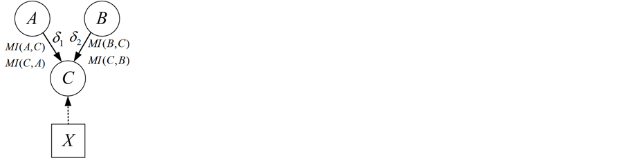
Figure 5. MI-QPN MI-QPN fragment.
Intuitively, the composition operator “Ú” ought to satisfy the following properties: 1) The composition weight belongs to [0, 1]; 2) The composition operation is commutative; 3) The composition operation is associative; 4) Combining two influences with the same qualitative signs (e.g., two “+” signs or two “−” signs) will result in an influence with a greater MI weight; 5) Combining two influences with different qualitative signs will result in an influence dependent on but less than the larger one. Inspired by the evidence theory and the basic idea of evidence combination [27] , we define the composition operator “Ú” based on evidence superposition.
Definition 5.1 , defined as follows:
・ if , then
 (15)
(15)
・ if
 and
and , then
 (16)
(16)
・ if
 and
and , then
 (17)
(17)
・ if
 and
and , then
 (18)
(18)
Based the above properties, we give Algorithm 2 for conflict-free inferences with the MI-QPN.
Now, we discuss the time complexity of Algorithm 2 for MI-QPN inferences. First, whether a node will be visited is determined by its node sign whose changes are specified in QPN’s general inference algorithm [8] , while the influence weights are just used to decide the node sign during inferences. Second, Algorithm 2 is the same as the general QPN’s inference algorithm if there does not exist “?” during inferences [8] . However, Algorithm 2 can be used to avoid the “?” results as possible by means of weighting influences quantitatively, where each time of weight computation w.r.t. the composition property can be fuelled by Step 5 in Merge-Sign in O(1) time. Therefore, the time complexity of Algorithm 2 will be the same as that for the general QPN’s inferences.
Algorithm 2.Conflict-free inference with an MI-QPN.
6. Experimental Results
To test the performance of our method in this paper, we implemented our algorithms for constructing and inferring MI-QPN. We take BN’s inference results obtained from Netica [28] as the criteria to decide whether the increase (or decrease) trends of the nodes indicated by the inference results of the corresponding MI-QPN are correct.
It is well known that Wet-Grass network is a classic BN for whether the Our Grass is wet, related to Our Wall, Rain, Our Sprinkler and Neighbor’s Grass status, containing 5 binary variables and 6 edges [2] [28] . From the Wet-Grass BN, we know the qualitative influences between node Rain and Neighbor’s Grass and the ones between Rain and Our Grass are the same. To illustrate our methods and show the results straightforwardly, we modify the knowledge in the network by removing node Neighbor’s Grass and the corresponding edge, which will not affect the rest part of the original network and we denote the possible values of the nodes wet, was on, rained as 1, and dry, was off, didn’t rain as 0. Moreover, we rename Our Wall as Wall or W, Our Grass as Grass or G and Our Sprinkler as Sprinkler or S for short. Then, the modified network is shown in Figure 6.
First, we derive the corresponding QPN and MI-QPN shown in Figure 7 and Figure 8 respectively. Then, we compare the inference results of the QPN and those of the MI-QPN to verify the feasibility of our algorithms. By using the general QPN’s inference algorithm [8] and our inference algorithm for an MI-QPN, we take each node in the QPN and the MI-QPN as evidence and record the inference results of other nodes. The comparisons are shown in Table 1, from which we can see all possible inference conflicts have been eliminated in the MI-QPN.
Then, we compare the inference results on the modified Wet-Grass BN and those on the derived MI-QPN. We take each node of the BN as evidence, and then record the inference results of other nodes shown in Table 2, where E-Node and E-Sign denotes the evidence and corresponding sign respectively. The E-sign 0 → 1 represents that the state of the evidence node changes from 0 to 1, indicating that the probability of state 1 is changed from 0 to 1. If a node in the MI-QPN takes sign “+” (“−”) as the final inference result and the increase (decrease) of the probability of state 1 of the corresponding node in the BN, we can conclude that the inference result is correct.
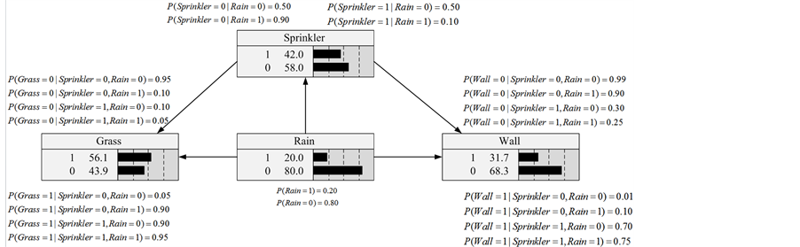
Figure 6. The modified Wet-Grass BN.
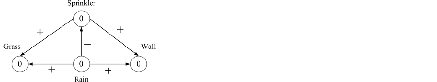
Figure 7. Wet-Grass QPN.
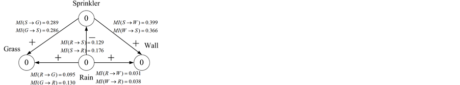
Figure 8. Wet-Grass MI-QPN.
Table 1. Comparisons of inference results between QPN and MI-QPN.
Table 2. Comparisons of inference results between the modified BN and the derived MI-QPN.
7. Conclusions and Future Work
In this paper, we introduced mutual-information based weights (MI weights) to qualitative influences in QPNs to resolve conflicts during the inferences. We first defined the MI weights based on mutual information and MI-QPN by extending the traditional QPN. Then, we proposed the method to derive the MI weights for the MI-QPN from the corresponding BN without sample data or threshold values. By theoretic analysis, we know the method for deriving MI weights is effective. Furthermore, we discussed the symmetry, transitivity and composition properties in the MI-QPN, and extended the general influence algorithm to implement the conflict-free inferences of MI-QPN. The feasibility of our method was verified by the results of the preliminary experiment.
Our work in this paper also leaves open some other interesting research issues. We are to further consider adding the MI weights to the qualitative synergies and discussing the method to resolve the inference conflicts caused by two inconsistent signs with the same MI weight. As well, we will further resolve the conflicts that take place during the fusion or integration of multiple QPNs by adding the MI weights to the qualitative influences in the QPNs. These are exactly our future work.
Acknowledgements
This work was supported by the National Natural Science Foundation of China (61472345), the Natural Science Foundation of Yunnan Province (2014FA023, 2013FA013), the Yunnan Provincial Foundation for Leaders of Disciplines in Science and Technology (2012HB004), and the Program for Innovative Research Team in Yunnan University (XT412011).
References
- Liu, W.Y., Li, W.H. and Yue, K. (2007) Intelligent Data Analysis. Science Press, Beijing.
- Pearl, J. (1988) Probabilistic Reasoning in Intelligent Systems: Network of Plausible Inference. Morgan Kaufmann, San Mateo.
- Li, W.H., Liu, W.Y. and Yue, K. (2008) Recovering the Global Structure from Multiple Local Bayesian Networks. International Journal on Artificial Intelligence Tools, 17, 1067-1088. http://dx.doi.org/10.1142/S0218213008004308
- Cooper, G.F. (1990) The Computational Complexity of Probabilistic Inference Using Bayesian Belief Networks. Artificial Intelligence, 42, 393-405. http://dx.doi.org/10.1016/0004-3702(90)90060-D
- Dagum, P. and Luby, M. (1993) Approximating Probabilistic Inference in Bayesian Belief Networks Is NP-Hard. Artificial Intelligence, 60, 141-153. http://dx.doi.org/10.1016/0004-3702(93)90036-B
- Wellman, M.P. (1990) Fundamental Concepts of Qualitative Probabilistic Networks. Artificial Intelligence, 44, 257- 303. http://dx.doi.org/10.1016/0004-3702(90)90026-V
- Bolt, J.H., Renooij, S. and Van der Gaag, L.C. (2003) Upgrading Ambiguous Signs in QPNs. Proceedings of the 19th Conference in Uncertainty in Artificial Intelligence, Acapulco, 7-10 August 2003, 73-80.
- Druzdzel, M.J. and Henrion, M. (1993) Efficient Reasoning in Qualitative Probabilistic Networks. Proceedings of the 11th National Conference on Artificial Intelligence, Washington DC, 11-15 July 1993, 548-553.
- Lv, Y.L. and Liao, S.Z. (2011) Ambiguity Reduction Based on Qualitative Mutual Information in Qualitative Probabilistic Networks. Pattern Recognition and Artificial Intelligence, 24, 123-129.
- Parsons, S. (1995) Refining Reasoning in Qualitative Probabilistic Networks. Proceedings of the 11th Conference on Uncertainty in Artificial Intelligence, Montreal, 18-20 August 1995, 427-434.
- Renooij, S., Parsons, S. and Pardieck, P. (2003) Using Kappas as Indicators of Strength in Qualitative Probabilistic Networks. Proceedings of European Conferences on Symbolic and Quantitative Approaches to Reasoning with Uncertainty, Aalborg, 2-5 July 2003, 87-99.
- Renooij, S. and Van der Gaag, L.C. (1999) Enhancing QPNs for Trade-Off Resolution. Proceedings of the 15th Conference on Uncertainty in Artificial Intelligence, Stockholm, 30 July-1 August 1999, 559-566.
- Renooij, S., Van der Gaag, L.C. and Parsons, S. (2002) Context-Specific Sign-Propagation in Qualitative Probabilistic Networks. Artificial Intelligence, 140, 207-230. http://dx.doi.org/10.1016/S0004-3702(02)00247-3
- Renooij, S., Van der Gaag, L.C., Parsons, S. and Green, S. (2000) Pivotal Pruning of Trade-Off in QPNs. Proceedings of the 16th Conference in Uncertainty in Artificial Intelligence, Stanford, 30 June-3 July 2000, 515-522.
- Renooij, S. and Van der Gaag, L.C. (2002) From Qualitative to Quantitative Probabilistic Network. Proceedings of the 18th Conference on Uncertainty in Artificial Intelligence, Edmonton, 1-4 August 2002, 422-429.
- Yue, K., Yao, Y., Li, J. and Liu, W.Y. (2010) Qualitative Probabilistic Networks with Reduced Ambiguities. Applied Intelligence, 33, 159-178. http://dx.doi.org/10.1007/s10489-008-0156-5
- Cover, T.M. and Thomas, J.A. (1993) Elements of Information Theory. John Wiley & Sons, Inc., Hoboken.
- Shannon, C.E. and Weaver, W. (1949) The Mathematical Theory of Communication. University of Illinois Press, Champaign.
- Chen, X.W., Anantha, G. and Lin, X.T. (2008) Improving Bayesian Network Structure Learning with Mutual Information-Based Node Ordering in the K2 Algorithm. IEEE Transactions on Knowledge and Data Engineering, 20, 628- 640. http://dx.doi.org/10.1109/TKDE.2007.190732
- De Campos, L.M. (2006) A Scoring Function for Learning Bayesian Networks Based on Mutual Information and Conditional Independence Tests. Journal of Machine Learning Research, 7, 2149-2187.
- Nicholson, A.E. and Jitnah, N. (1998) Using Mutual Information to Determine Relevance in Bayesian Networks. Proceedings of the 5th Pacific Rim International Conference on Artificial Intelligence, Singapore, 22-27 November 1998, 399-410.
- Ibrahim, Z.M., Ngom, A. and Tawk, A.Y. (2011) Using Qualitative Probability in Reverse-Engineering Gene Regulatory Networks. IEEE/ACM Transactions on Computational Biology and Bioinformatics, 8, 326-334. http://dx.doi.org/10.1109/TCBB.2010.98
- Liu, W.Y., Yue, K., Liu, S.X. and Sun, Y.B. (2008) Qualitative-Probabilistic-Network-Based Modeling of Temporal Causalities and Its Application to Feedback Loop Identification. Information Sciences, 178, 1803-1824. http://dx.doi.org/10.1016/j.ins.2007.11.021
- Yue, K., Qian, W.H., Fu, X.D., Li, J. and Liu, W.Y. (2014) Qualitative-Probabilistic-Network-Based Fusion of Time- Series Uncertain Knowledge. Soft Computing, Published Online. http://dx.doi.org/10.1007/s00500-014-1381-y.
- De Campos, C.P. and Cozman, F.G. (2013) Complexity of Inferences in Polytree-Shaped Semi-Qualitative Probabilistic Networks. Proceedings of the 27th AAAI Conference on Artificial Intelligence, Bellevue, 14-18 July 2013, 217-223.
- Yue, K., Liu, W. and Yue, M. (2011) Quantifying Influences in the Qualitative Probabilistic Network with Interval Probability Parameters. Applied Soft Computing, 11, 1135-1143. http://dx.doi.org/10.1016/j.asoc.2010.02.013
- Shafer, G. (1986) The Combination of Evidence. International Journal of Intelligent Systems, 1, 155-179. http://dx.doi.org/10.1002/int.4550010302
- Norsys Software Corp. (2007) Netica 3.17 Bayesian Network Software from Norsys. http://www.norsys.com